Fill in Blanks
Home
1.1 Bivariate Relationships
1.2 Probabilistic Models
1.3 Estimation of the Line
1.4 Properties of the Least Squares Estimators
1.5 Estimation of the Variance
2.1 The Normal Errors Model
2.2 Inferences for the Slope
2.3 Inferences for the Intercept
2.4 Correlation and Coefficient of Determination
2.5 Estimating the Mean Response
2.6 Predicting the Response
3.1 Residual Diagnostics
3.2 The Linearity Assumption
3.3 Homogeneity of Variance
3.4 Checking for Outliers
3.5 Correlated Error Terms
3.6 Normality of the Residuals
4.1 More Than One Predictor Variable
4.2 Estimating the Multiple Regression Model
4.3 A Primer on Matrices
4.4 The Regression Model in Matrix Terms
4.5 Least Squares and Inferences Using Matrices
4.6 ANOVA and Adjusted Coefficient of Determination
4.7 Estimation and Prediction of the Response
5.1 Multicollinearity and Its Effects
5.2 Adding a Predictor Variable
5.3 Outliers and Influential Cases
5.4 Residual Diagnostics
5.5 Remedial Measures
7.4 Lasso
"You want the moon? Just say the word, and I'll throw a lasso around it and pull it down."
- George Bailey (It's a Wonderful Life )
Recall in Section 5.5.4 that ridge regression can be used as a remedial measure when there is multicollinearity in the model.
The variables are first transformed using the correlation transformation in (5.23)
The estimates are then found by minimizing \begin{align*} Q & =\sum\left[Y_{i}^{*}-\left(b_{1}^{*}X_{i1}^{*}+\cdots+b_{p-1}^{*}X_{i,p-1}^{*}\right)\right]^{2}+\lambda\left[\sum_{j=1}^{p-1}\left(b_{j}^{*}\right)^{2}\right]\qquad(5.24) \end{align*} These estimatesshrink to zero for predictors that do not have a significant linear relationship on $Y$ given the other variables.
In ridge regression, the coefficient estimates shrink to zero, but do not equal zero.
The variables are first transformed using the correlation transformation in (5.23)
\begin{align*}
Y_{i}^{*} & =\frac{1}{\sqrt{n-1}}\left(\frac{Y_{i}-\overline{Y}}{s_{Y}}\right)\\
X_{ik}^{*} & =\frac{1}{\sqrt{n-1}}\left(\frac{X_{ik}-\overline{X}_{k}}{s_{k}}\right)\qquad(5.23)
\end{align*}
.
The estimates are then found by minimizing \begin{align*} Q & =\sum\left[Y_{i}^{*}-\left(b_{1}^{*}X_{i1}^{*}+\cdots+b_{p-1}^{*}X_{i,p-1}^{*}\right)\right]^{2}+\lambda\left[\sum_{j=1}^{p-1}\left(b_{j}^{*}\right)^{2}\right]\qquad(5.24) \end{align*} These estimates
In ridge regression, the coefficient estimates shrink to zero, but do not equal zero.
The lasso (least absolute shrinkage and selection operator ) is a shrinkage method like ridge, with subtle but important differences.
The lasso estimate is defined by \begin{align*} Q_{lasso} & =\sum_{i=1}^{n}\left(Y_{i}-\left(\beta_{0}+\beta_{1}X_{1i}+\cdots+\beta_{p-1}X_{p-1,i}\right)\right)^{2}+\lambda\sum_{j=1}^{p-1}\left|\beta_{j}\right| \qquad (7.9) \end{align*} Similarly to ridge regression, the lasso can also be rewritten to be minimizing the sums of squares subject to the sum of the absolute values of the non-intercept beta coefficients being less than a constraint $\tau$: \begin{align*} \sum_{j=1}^{p-1}|\beta_{j}| & \le\tau \qquad (7.10) \end{align*} As $\tau$ decreases toward 0, the beta coefficients shrink toward zero with the least associated beta coefficients decreasing all the way to 0 before the more strongly associated beta coefficients.
As a result, numerous beta coefficients that are not strongly associated with the outcome are decreased to zero, which is equivalent to removing those variables from the model.
In this way, the lasso can be used as a variable selection method.
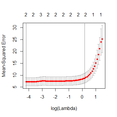
In order to find the optimal $\lambda$, a range of $\lambda$'s are tested, with the optimal $\lambda$ chosen using a cross-validation.
The lasso estimate is defined by \begin{align*} Q_{lasso} & =\sum_{i=1}^{n}\left(Y_{i}-\left(\beta_{0}+\beta_{1}X_{1i}+\cdots+\beta_{p-1}X_{p-1,i}\right)\right)^{2}+\lambda\sum_{j=1}^{p-1}\left|\beta_{j}\right| \qquad (7.9) \end{align*} Similarly to ridge regression, the lasso can also be rewritten to be minimizing the sums of squares subject to the sum of the absolute values of the non-intercept beta coefficients being less than a constraint $\tau$: \begin{align*} \sum_{j=1}^{p-1}|\beta_{j}| & \le\tau \qquad (7.10) \end{align*} As $\tau$ decreases toward 0, the beta coefficients shrink toward zero with the least associated beta coefficients decreasing all the way to 0 before the more strongly associated beta coefficients.
As a result, numerous beta coefficients that are not strongly associated with the outcome are decreased to zero, which is equivalent to removing those variables from the model.
In this way, the lasso can be used as a variable selection method.
In order to find the optimal $\lambda$, a range of $\lambda$'s are tested, with the optimal $\lambda$ chosen using a cross-validation.
Because the lasso estimates are biased, then examining the standard errors of the estimators do not give the whole picture. The standard errors might be small but we must remember these estimates are biased.
Because of this, confidence intervals and prediction intervals are not easily interpreted.
If prediction intervals are desired, one could use lasso to select the predictor variables and then fit that model using ordinary least squares. This is briefly mentioned in Section 11.4 of Hastie, Tibshirani, Wainwright (2015)
Hastie, T., Tibshirani, R., & Wainwright, M. (2015). Statistical learning with sparsity: the lasso and generalizations. Chapman and Hall/CRC.
.
In Example 5.5.5 we used ridge regression on the body fat data due to the multicollinearity among the predictor variables.
We will now use the lasso procedure to select the model.
It is important to note that when two $X$ variables are highly correlated, the lasso will arbitrarily have one of those variables shrink to zero. The practitioner should understand that the one variable that was not selected could in fact be more appropriate for their model than the one that was selected.
We will now use the lasso procedure to select the model.
library(tidyverse)
library(car)
library(olsrr)
library(MASS)
library(glmnet)
dat = read.table("http://www.jpstats.org/Regression/data/BodyFat.txt", header=T)
#for cv.glmnet, you must input the variables as matrices
X = dat[,1:3] %>% as.matrix()
y = dat[,4] %>% as.matrix()
#must specify alpha=1 for lasso
fit.lasso = cv.glmnet(X, y, alpha=1)
#plot the mean square error for different lambdas
plot(fit.lasso)
 #we can obtain the lasso estimates
predict(fit.lasso, s ="lambda.min", type = "coefficients")
#we can obtain the lasso estimates
predict(fit.lasso, s ="lambda.min", type = "coefficients")
4 x 1 sparse Matrix of class "dgCMatrix"
1
(Intercept) 6.7197922
tri 0.9949266
thigh .
midarm -0.4236571
It is important to note that when two $X$ variables are highly correlated, the lasso will arbitrarily have one of those variables shrink to zero. The practitioner should understand that the one variable that was not selected could in fact be more appropriate for their model than the one that was selected.