5.2 Adding a Predictor Variable

We have seen that plotting the residuals vs a predictor variable in Section 3.2.1 is one way to determine if a linear relationship in the simple linear regression model is adequate.

If the points in this plot were not just randomly scattered about zero, then a model incorporating the nonlinear relationship may be needed.

Likewise, we can plot the residuals vs each predictor variable in multiple regression. Again, this shows if a linear term for that predictor variable is adequate in our model or if nonlinear term is needed.

We can also plot the residuals vs a potential predictor variable that is not already in the model. Any systematic pattern in this residual plot indicates that potential $X$ variables may be useful in modeling $Y$.

A residual plot vs a potential $X$ is limited in that it may not show the marginal effect of adding that variable when all other variables are already added. To see the marginal effect, we will need a different plot.

To see the marginal importance of a potential $X_{j}$ on modeling $Y$, given the other predictor variables that are already in the model, we can regression $X_{j}$ on all the predictor variables already in the model.

We then find the residuals of this fit which we denote as $e_{X_{j}|{\bf X}}$.

We now plot the residuals from the model involving $Y$ (regressed on the predictor variables not including $X_{j}$) against $e_{X_{j}|{\bf X}}$.

This plot is called an added variable plot. It is also sometimes called a partial regression plot or an adjusted variable plot.

From the added variable plot we can see the marginal importance of $X_{j}$ in reducing the variability remaining after regression on the other predictor variables. If the plot shows the points in a linear pattern with a nonzero slope, then $X_{j}$ may be helpful in explaining more variability in $Y$ in addition to the variables already included.

We may also see a systematic but nonlinear patter in the points. This means $X_{j}$ maybe helpful in the model but a nonlinear term is needed.

Let's examine the bodyfat data once again.

library(tidyverse)
library(car)

dat = read.table("http://www.jpstats.org/Regression/data/BodyFat.txt", header=T)

#suppose we start with just thigh in the model
fit2 = lm(bfat~thigh, data=dat)

dat$res2 = fit2 %>% resid()

#plot the residuals versus the potential variable tri
ggplot(dat, aes(x=tri, y=res2))+
  geom_point()




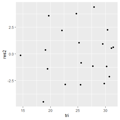
#this plots shows no systematic pattern so a nonlinear term is 
#not needed. However, does tri add explain anything more about
#Y given thigh is already included

#fit the model with both
fit12 = lm(bfat~tri+thigh, data=dat)

#give the added variable plots for all variables
#in the fit
avPlots(fit12)




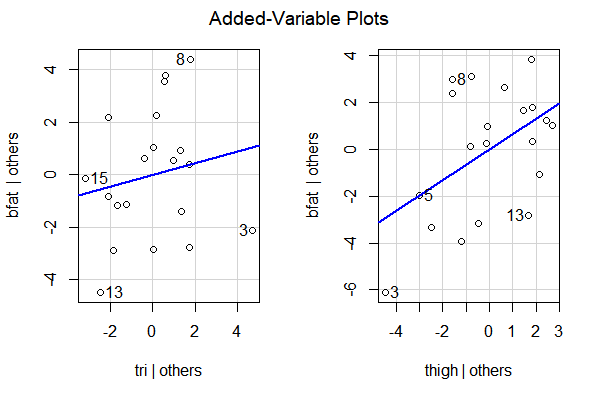
# It appears adding thigh when tri is already included helps more 
# than including tri when thigh is already included. This is
# because the plots show thigh with a steeper slope and less
# spread about the line