Fill in Blanks
Home
1.1 Bivariate Relationships
1.2 Probabilistic Models
1.3 Estimation of the Line
1.4 Properties of the Least Squares Estimators
1.5 Estimation of the Variance
2.1 The Normal Errors Model
2.2 Inferences for the Slope
2.3 Inferences for the Intercept
2.4 Correlation and Coefficient of Determination
2.5 Estimating the Mean Response
2.6 Predicting the Response
3.1 Residual Diagnostics
3.2 The Linearity Assumption
3.3 Homogeneity of Variance
3.4 Checking for Outliers
3.5 Correlated Error Terms
3.6 Normality of the Residuals
4.1 More Than One Predictor Variable
4.2 Estimating the Multiple Regression Model
4.3 A Primer on Matrices
4.4 The Regression Model in Matrix Terms
4.5 Least Squares and Inferences Using Matrices
4.6 ANOVA and Adjusted Coefficient of Determination
4.7 Estimation and Prediction of the Response
5.1 Multicollinearity and Its Effects
5.2 Adding a Predictor Variable
5.3 Outliers and Influential Cases
5.4 Residual Diagnostics
5.5 Remedial Measures
6.1 Indicator Variables
"Not everything that can be counted counts, and not everything that counts can be counted."
- Albert Einstein
Thus far, we have only considered predictor variables that are quantitative.
Qualitative predictor variables can also be used in regression models.
For example, consider the handspan data first examined in Section 1.1.1. We can regress the handspan on height but it will also make sense to include sex as well. We expect that males will tend to have a handspan larger than that of females.
In Figure 6.1.1 below, we plot handspan vs height and color females with red and males with blue. The least squares fit for each group are also shown.
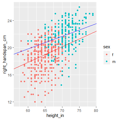
We can see that sex plays a role in the regression line. For the male subjects, the fitted line tends to be higher than for the female subjects.
Qualitative predictor variables can also be used in regression models.
For example, consider the handspan data first examined in Section 1.1.1. We can regress the handspan on height but it will also make sense to include sex as well. We expect that males will tend to have a handspan larger than that of females.
In Figure 6.1.1 below, we plot handspan vs height and color females with red and males with blue. The least squares fit for each group are also shown.
Figure 6.1.1: Handspan and Height by Sex
We can see that sex plays a role in the regression line. For the male subjects, the fitted line tends to be higher than for the female subjects.
We will include the qualitative variables in our model by using indicator variables.
An indicator variable (ordummy variable) takes on the values of 0
and 1. For example, a model for the handspan data is
\begin{align*}
Y_{i} & =\beta_{0}+\beta_{1}X_{i1}+\beta_{2}X_{i2}+\varepsilon
\end{align*}
where
\begin{align*}
Y & =\text{ handspan}\\
X_{1} & =\text{ height}\\
X_{2} & =\begin{cases}
1 & \text{ if sex=M}\\
0 & \text{ otherwise}
\end{cases}
\end{align*}
An indicator variable (or
If the subject is male, then the expectation becomes
\begin{align*}
E\left[Y_{i}\right] & =\beta_{0}+\beta_{1}X_{i1}+\beta_{2}\left(1\right)\\
& =\left(\beta_{0}+\beta_{2}\right)+\beta_{1}X_{i1}
\end{align*}
If the subject is female, the expectation is
\begin{align*}
E\left[Y_{i}\right] & =\beta_{0}+\beta_{1}X_{i1}+\beta_{2}\left(0\right)\\
& =\beta_{0}+\beta_{1}X_{i1}
\end{align*}
Thus, the two groups will have the same slope ($\beta_{1}$), but will have different intercepts. That means the means of the two groups are different by $\beta_{2}$ for all values of $X_{1}$.
We could also have different slopes for the two groups. We will discuss this in Section 6.2.
Thus, the two groups will have the same slope ($\beta_{1}$), but will have different intercepts. That means the means of the two groups are different by $\beta_{2}$ for all values of $X_{1}$.
We could also have different slopes for the two groups. We will discuss this in Section 6.2.
Let's examine the handspan data.
library(tidyverse)
library(car)
library(olsrr)
library(MASS)
library(glmnet)

dat = read.table("http://www.jpstats.org/Regression/data/Survey_Measurements.csv",sep=",", header=T)
#when reading in data using read.table, any variable that is not a number is
#treated as a factor. A factor is a qualitative variable in R

#the lm function will take a factor and automatically create an indicator variable
fit = lm(right_handspan_cm~height_in+sex, data=dat)

fit %>% summary

Call:
lm(formula = right_handspan_cm ~ height_in + sex, data = dat)

Residuals:
    Min      1Q  Median      3Q     Max
-7.1077 -1.1709  0.3311  1.3088  4.1020

Coefficients:
            Estimate Std. Error t value Pr(>|t|)
(Intercept)  5.10972    1.44120   3.545 0.000414 ***
height_in    0.21314    0.02218   9.611   2e-16 ***
sexm         1.63165    0.18319   8.907   2e-16 ***
---
Signif. codes:  0 ‘***’ 0.001 ‘**’ 0.01 ‘*’ 0.05 ‘.’ 0.1 ‘ ’ 1

Residual standard error: 1.92 on 831 degrees of freedom
Multiple R-squared:  0.3855,	Adjusted R-squared:  0.3841
F-statistic: 260.7 on 2 and 831 DF,  p-value:  2.2e-16


#note that the variable sex has an m next to it. This is letting
#you know that m (male) is variable encoded with 1.
#the first level is called the reference level, here the
#reference level is f

#if you would rather have female encode with 1, then we would need to
#change the reference level to m in the data set
dat$sex = relevel(dat$sex, ref = "m")
fit2 = lm(right_handspan_cm~height_in+sex, data=dat)
fit2 %>% summary

Call:
lm(formula = right_handspan_cm ~ height_in + sex, data = dat)

Residuals:
    Min      1Q  Median      3Q     Max
-7.1077 -1.1709  0.3311  1.3088  4.1020

Coefficients:
            Estimate Std. Error t value Pr(>|t|)
(Intercept)  6.74137    1.56514   4.307 1.85e-05 ***
height_in    0.21314    0.02218   9.611   2e-16 ***
sexf        -1.63165    0.18319  -8.907   2e-16 ***
---
Signif. codes:  0 ‘***’ 0.001 ‘**’ 0.01 ‘*’ 0.05 ‘.’ 0.1 ‘ ’ 1

Residual standard error: 1.92 on 831 degrees of freedom
Multiple R-squared:  0.3855,	Adjusted R-squared:  0.3841
F-statistic: 260.7 on 2 and 831 DF,  p-value:  2.2e-16


#note that the coefficient for sex is now a negative
#also, the slope did not change.
We can use indicator variables for qualitative predictors that have more than two classes (categories).
For example, suppose we wanted to model the sales price of a home bases on the quantitative predictors lot size ($X_1$), local taxes ($X_2$), and age ($X_3$).
We may also want to include the qualitative predictor for air conditioning type. The possible classes are "no air conditioning", "window units", "heat pumps", and "central air conditioning".
We will now set up the indicator variables in the following way: \begin{align*} X_{4} & =\begin{cases} 1 & \text{ if no air conditioning}\\ 0 & \text{ otherwise } \end{cases}\\ X_{5} & =\begin{cases} 1 & \text{ if window units}\\ 0 & \text{ otherwise } \end{cases}\\ X_{6} & =\begin{cases} 1 & \text{ if heat pumps}\\ 0 & \text{ otherwise } \end{cases} \end{align*} We do not include an indicator variable for the last class ``central air conditioning'' because subjects with $X_{4}=0$, $X_{5}=0$, and $X_{6}=0$ will be considered in the class ``central air conditioning''.
As a general rule, if there are $c$ classes for a qualitative variable, then $c-1$ indicator variables will be needed.
The expectations become \begin{align*} \text{no air conditioning: }E\left[Y_{i}\right]= & \beta_{0}+\beta_{1}X_{i1}+\beta_{2}X_{i2}+\beta_{3}X_{i3}+\beta_{4}\left(1\right)+\beta_{5}\left(0\right)+\beta_{6}\left(0\right)\\ = & \left(\beta_{0}+\beta_{4}\right)+\beta_{1}X_{i1}+\beta_{2}X_{i2}+\beta_{3}X_{i3} \end{align*} \begin{align*} \text{window units: }E\left[Y_{i}\right]= & \beta_{0}+\beta_{1}X_{i1}+\beta_{2}X_{i2}+\beta_{3}X_{i3}+\beta_{4}\left(0\right)+\beta_{5}\left(1\right)+\beta_{6}\left(0\right)\\ = & \left(\beta_{0}+\beta_{5}\right)+\beta_{1}X_{i1}+\beta_{2}X_{i2}+\beta_{3}X_{i3} \end{align*} \begin{align*} \text{heat pumps: }E\left[Y_{i}\right]= & \beta_{0}+\beta_{1}X_{i1}+\beta_{2}X_{i2}+\beta_{3}X_{i3}+\beta_{4}\left(0\right)+\beta_{5}\left(0\right)+\beta_{6}\left(1\right)\\ = & \left(\beta_{0}+\beta_{6}\right)+\beta_{1}X_{i1}+\beta_{2}X_{i2}+\beta_{3}X_{i3} \end{align*} \begin{align*} \text{central air conditioning: }E\left[Y_{i}\right]= & \beta_{0}+\beta_{1}X_{i1}+\beta_{2}X_{i2}+\beta_{3}X_{i3}+\beta_{4}\left(0\right)+\beta_{5}\left(0\right)+\beta_{6}\left(0\right)\\ = & \beta_{0}+\beta_{1}X_{i1}+\beta_{2}X_{i2}+\beta_{3}X_{i3} \end{align*} So once again the slopes will be the same for each class but the intercept will change for different classes.
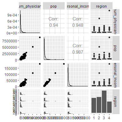
Let's examine the CDI data from Kutner
Kutner, M. H., Nachtsheim, C. J., Neter, J., & Li, W. (2005). Applied linear statistical models (Vol. 5). Boston: McGraw-Hill Irwin.
. The data consist of the number of active physicians ($Y$), the population size, total personal income, and region of
440 counties in the United States.
library(tidyverse)
library(car)
library(olsrr)
library(MASS)
library(glmnet)
library(GGally)
dat = read.table("http://www.jpstats.org/Regression/data/CDI.txt", header=T)
#the variable region is currently coded as
# 1 - New England
# 2 - North Central
# 3 - Southern
# 4 - Western
#notice that R reads these as integers and not factors.
#if you include these in the lm function, then they
# will be treated as any other quantitative variable
#We could tell R to make region a factor in the dataset:
dat$region = as.factor(dat$region)
#now region would be treated as a factor in lm
#let's examine these variables
ggpairs(dat[,c(8, 5, 16, 17)])
#We could also tell lm to treat as a factor:
fit = lm(num_physicians~pop+personal_income+factor(region), data=dat)
fit %>% summary
Call:
lm(formula = num_physicians ~ pop + personal_income + factor(region),
data = dat)
Residuals:
Min 1Q Median 3Q Max
-1866.8 -207.7 -81.5 72.4 3721.7
Coefficients:
Estimate Std. Error t value Pr(>|t|)
(Intercept) -5.848e+01 5.882e+01 -0.994 0.3207
pop 5.515e-04 2.835e-04 1.945 0.0524 .
personal_income 1.070e-01 1.325e-02 8.073 6.8e-15 ***
factor(region)2 -3.493e+00 7.881e+01 -0.044 0.9647
factor(region)3 4.220e+01 7.402e+01 0.570 0.5689
factor(region)4 -1.490e+02 8.683e+01 -1.716 0.0868 .
---
Signif. codes: 0 ‘***’ 0.001 ‘**’ 0.01 ‘*’ 0.05 ‘.’ 0.1 ‘ ’ 1
Residual standard error: 566.1 on 434 degrees of freedom
Multiple R-squared: 0.9011, Adjusted R-squared: 0.8999
F-statistic: 790.7 on 5 and 434 DF, p-value: 2.2e-16
#if we want to see what the design matrix X would look like:
X = model.matrix(fit)
X
(Intercept) pop personal_income factor(region)2 factor(region)3 factor(region)4
1 1 8863164 184230 0 0 1
2 1 5105067 110928 1 0 0
3 1 2818199 55003 0 1 0
4 1 2498016 48931 0 0 1
5 1 2410556 58818 0 0 1
6 1 2300664 38658 0 0 0
7 1 2122101 38287 0 0 1
8 1 2111687 36872 1 0 0
9 1 1937094 34525 0 1 0
10 1 1852810 38911 0 1 0
11 1 1585577 26512 0 0 0
12 1 1507319 35843 0 0 1
13 1 1497577 37728 0 0 1
14 1 1418380 23260 0 0 1
15 1 1412140 29776 1 0 0
#use the matrix form of the least squares
solve(t(X)%*%X)%*%t(X)%*%dat[,8]
[,1]
(Intercept) -5.847618e+01
pop 5.514599e-04
personal_income 1.070115e-01
factor(region)2 -3.493126e+00
factor(region)3 4.219673e+01
factor(region)4 -1.490196e+02
#We will discuss more about which predictors should be
#included in the model in Chapter 7
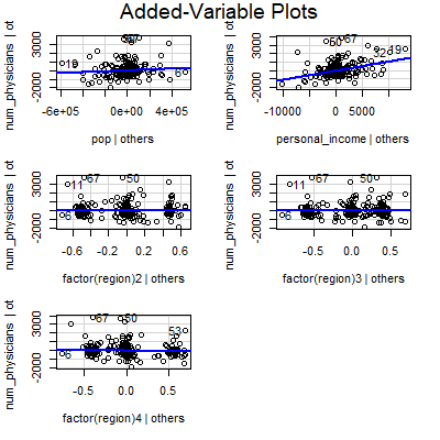
#for now, we could examine the added variable plots
#as before, we look for a significant slope in the line in the
#added variable plot
avPlots(fit)
#if you only want to include one of the classes, ie class 3 or otherwise,
#then you can use the I function in lm
fit1 = lm(num_physicians~pop+personal_income+I(region=="3"), data=dat)
fit1 %>% summary
Call:
lm(formula = num_physicians ~ pop + personal_income + I(region ==
"3"), data = dat)
Residuals:
Min 1Q Median 3Q Max
-1832.2 -202.1 -67.5 47.2 3761.1
Coefficients:
Estimate Std. Error t value Pr(>|t|)
(Intercept) -9.434e+01 3.867e+01 -2.440 0.0151 *
pop 4.818e-04 2.792e-04 1.725 0.0852 .
personal_income 1.098e-01 1.307e-02 8.401 6.3e-16 ***
I(region == "3")TRUE 8.393e+01 5.757e+01 1.458 0.1456
---
Signif. codes: 0 ‘***’ 0.001 ‘**’ 0.01 ‘*’ 0.05 ‘.’ 0.1 ‘ ’ 1
Residual standard error: 567.2 on 436 degrees of freedom
Multiple R-squared: 0.9002, Adjusted R-squared: 0.8996
F-statistic: 1311 on 3 and 436 DF, p-value: 2.2e-16