Fill in Blanks
Home
1.1 Bivariate Relationships
1.2 Probabilistic Models
1.3 Estimation of the Line
1.4 Properties of the Least Squares Estimators
1.5 Estimation of the Variance
2.1 The Normal Errors Model
2.2 Inferences for the Slope
2.3 Inferences for the Intercept
2.4 Correlation and Coefficient of Determination
2.5 Estimating the Mean Response
2.6 Predicting the Response
3.1 Residual Diagnostics
3.2 The Linearity Assumption
3.3 Homogeneity of Variance
3.4 Checking for Outliers
3.5 Correlated Error Terms
3.6 Normality of the Residuals
4.1 More Than One Predictor Variable
4.2 Estimating the Multiple Regression Model
4.3 A Primer on Matrices
4.4 The Regression Model in Matrix Terms
4.5 Least Squares and Inferences Using Matrices
4.6 ANOVA and Adjusted Coefficient of Determination
4.7 Estimation and Prediction of the Response
5.1 Multicollinearity and Its Effects
5.2 Adding a Predictor Variable
5.3 Outliers and Influential Cases
5.4 Residual Diagnostics
5.5 Remedial Measures
1.3 Estimation of the Line
"Regression. It is a universal rule that the unknown kinsman in any degree of any specified man, is probably more mediocre than he." - Francis Galton
The first step in regression analysis is to plot the $(X_i,Y_i)$ data values in a scatterplot. From this, you see what type of funtion would best describe the relationship between $X$ and $Y$.
In most situations, the data you have will be from asample .
Suppose you plot the data in a scatterplot and you determine that a linear function would best describe the relationship.
We will find the line that "best " fits the data. The intercept and slope of this fitted line will be estimates of the intercept ($\beta_0$) and slope ($\beta_1$) parameters in model (1.1)
We now need to define what is meant by "best" line.
In most situations, the data you have will be from a
Suppose you plot the data in a scatterplot and you determine that a linear function would best describe the relationship.
We will find the line that "
$$
Y_i=\beta_0+\beta_1X_i+\varepsilon_i\qquad\qquad\qquad(1.1)
$$
We now need to define what is meant by "best" line.
In model (1.1)
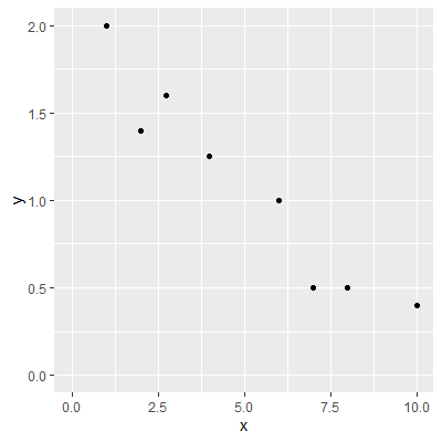
For example, suppose we have the data presented in the table to the right and plotted in the scatterplot in Figure 1.3.1 below.
We want the line that will be closest to the observed $Y_i$ values. Since the $Y$ variable is represented by the vertical axis on the plot, we want a line that makes all of thevertical distances between the points and the line as small as possible.
$$
Y_i=\beta_0+\beta_1X_i+\varepsilon_i\qquad\qquad\qquad(1.1)
$$
, we are interested in modeling the variable $Y$ based on $X$. Because of this, the line that "best" fits the data should be judged based on how well it "models" the observed $Y_i$ values.
For example, suppose we have the data presented in the table to the right and plotted in the scatterplot in Figure 1.3.1 below.
We want the line that will be closest to the observed $Y_i$ values. Since the $Y$ variable is represented by the vertical axis on the plot, we want a line that makes all of the
$$
Y_i=\beta_0+\beta_1X_i+\varepsilon_i\qquad\qquad\qquad(1.1)
$$
.
Any points below the line ($\hat Y$) will have a
For the data in Table 1.3.1, the scatterplot is presented in Figure 1.3.1 to the right.
Use your mouse and click any two spots on the scatterplot. A line will be drawn between through the two spots you click. The fitted values $\hat{Y_i}$, the distances $\left(Y_i-\hat{Y}_i\right)$, and the squared distances $\left(Y_i-\hat{Y}_i\right)^2$ are shown in Table 1.3.2 for the line you constructed.
The estimated line is
$$
\hat{Y}=\hat{\beta}_0+\hat{\beta}_1X
$$
Clicking on the plot a third time will clear the line.
You can then try another two points.
Try to get the sum of the squared distances
smaller by trying different lines.
Figure 1.3.1: Scatterplot of Data
For ease of notation, we will not include the starting and ending index in the summations going forward when the starting index is $i=1$ and the ending index is $n$. When the indices is something other than $i=1$ and $n$, then the indices will be included on the summation.
We will denote the sum of the squared distances with $Q$: $$ \begin{align*} Q&=\sum \left(Y_i-\hat{Y}_i\right)^2 \qquad\qquad\qquad (1.2) \end{align*} $$ We determine the "best" line as the one that minimizes $Q$. We will denote the intercept and slope of the line that minimize $Q$, given the data $(X_i, Y_i)$, $i=1,\ldots, n$, as $b_0$ and $b_1$, respectively.
To minimize $Q$, we differentiate it with respect to $b_{0}$ and $b_{1}$: \begin{align*} \frac{\partial Q}{\partial b_{0}} & =-2\sum \left(Y_{i}-\left(b_{0}+b_{1}X_{i}\right)\right)\\ \frac{\partial Q}{\partial b_{1}} & =-2\sum X_{i}\left(Y_{i}-\left(b_{0}+b_{1}X_{i}\right)\right) \end{align*} Setting these partial derivatives equal to 0, we have \begin{align*} -2\sum \left(Y_{i}-\left(b_{0}+b_{1}X_{i}\right)\right) & =0\\ -2\sum X_{i}\left(Y_{i}-\left(b_{0}+b_{1}X_{i}\right)\right) & =0 \end{align*} Looking at the first equation, we can simplify as \begin{align*} -2\sum \left(Y_{i}-\left(b_{0}+b_{1}X_{i}\right)\right)=0 & \Longrightarrow\sum \left(Y_{i}-\left(b_{0}+b_{1}X_{i}\right)\right)=0\\ & \Longrightarrow\sum Y_{i}-\sum b_{0}-b_{1}\sum X_{i}=0\\ & \Longrightarrow\sum Y_{i}-nb_{0}-b_{1}\sum X_{i}=0\\ & \Longrightarrow\sum Y_{i}=nb_{0}+b_{1}\sum X_{i} \end{align*} Simplifying the second equation gives us \begin{align*} -2\sum X_{i}\left(Y_{i}-\left(b_{0}+b_{1}X_{i}\right)\right)=0 & \Longrightarrow\sum X_{i}\left(Y_{i}-\left(b_{0}+b_{1}X_{i}\right)\right)=0\\ & \Longrightarrow\sum X_{i}Y_{i}-b_{0}\sum X_{i}-b_{1}\sum X_{i}^{2}=0\\ & \Longrightarrow\sum X_{i}Y_{i}=b_{0}\sum X_{i}+b_{1}\sum X_{i}^{2} \end{align*} The two equations \begin{align*} \sum Y_{i} & =nb_{0}+b_{1}\sum X_{i}\\ \sum X_{i}Y_{i} & =b_{0}\sum X_{i}+b_{1}\sum X_{i}^{2}\qquad\qquad\qquad(1.3) \end{align*} are called the
We now have two equations and two unknowns ($b_{0}$ and $b_{1}$). We can solve the equations simultaneously. We solve the first equation for $b_{0}$ which gives us \begin{align*} b_{0} & =\frac{1}{n}\left(\sum Y_{i}-b_{1}\sum X_{i}\right)\\ & =\bar{Y}-b_{1}\bar{X}. \end{align*} We now substitute this into the second equation in (1.3). Solving this for $b_{1}$ gives us (complete solution here
\begin{align*}
& \sum X_{i}Y_{i}=b_{0}\sum X_{i}+b_{1}\sum X_{i}^{2}\\
& \quad\Longrightarrow\sum X_{i}Y_{i}=\left(\bar{Y}-b_{1}\bar{X}\right)\sum X_{i}+b_{1}\sum X_{i}^{2}\\
& \quad\Longrightarrow\sum X_{i}Y_{i}=\bar{Y}\sum X_{i}-b_{1}\bar{X}\sum X_{i}+b_{1}\sum X_{i}^{2}\\
& \quad\Longrightarrow\sum X_{i}Y_{i}-\bar{Y}\sum X_{i}=\left(\sum X_{i}^{2}-\bar{X}\sum X_{i}\right)b_{1}\\
& \quad\Longrightarrow\sum X_{i}Y_{i}-\bar{Y}\sum X_{i}\underbrace{-\bar{X}\sum Y+\bar{X}\sum Y}_{\text{completing the square}}=\left(\sum X_{i}^{2}-\bar{X}\sum X_{i}\underbrace{-\bar{X}\sum X+\bar{X}\sum X}_{\text{completing the square}}\right)b_{1}\\
& \quad\Longrightarrow\sum \left(X_{i}-\bar{X}\right)\left(Y_{i}-\bar{Y}\right)=\left(\sum \left(X_{i}-\bar{X}\right)^{2}\right)b_{1}\\
& \quad\Longrightarrow b_{1}=\frac{\sum \left(X_{i}-\bar{X}\right)\left(Y_{i}-\bar{Y}\right)}{\sum \left(X_{i}-\bar{X}\right)^{2}}.
\end{align*}
):
\begin{align*}
& \sum X_{i}Y_{i}=b_{0}\sum X_{i}+b_{1}\sum X_{i}^{2}\\
& \quad\Longrightarrow\sum X_{i}Y_{i}=\left(\bar{Y}-b_{1}\bar{X}\right)\sum X_{i}+b_{1}\sum X_{i}^{2}\\
&\quad\Longrightarrow b_{1}=\frac{\sum \left(X_{i}-\bar{X}\right)\left(Y_{i}-\bar{Y}\right)}{\sum \left(X_{i}-\bar{X}\right)^{2}}.
\end{align*}
The equations
\begin{align*}
b_{0} & =\bar{Y}-b_{1}\bar{X}\\
b_{1} & =\frac{\sum \left(X_{i}-\bar{X}\right)\left(Y_{i}-\bar{Y}\right)}{\sum \left(X_{i}-\bar{X}\right)^{2}}\qquad\qquad\qquad(1.4)
\end{align*}
are called the To show these estimators are the minimum, we take the second partial derivatives of $Q$: \begin{align*} \frac{\partial^{2}Q}{\partial\left(b_{0}\right)^{2}} & =2n\\ \frac{\partial^{2}Q}{\partial\left(b_{1}\right)^{2}} & =2\sum X_{i}^{2} \end{align*} Since these second partial derivatives are both positives, then we know the least squares estimators are the minimum.
We now use R to find the least squares estimates for the line that best fits the data in Table 1.3.1
. We first load in the data, convert to a tibble, and then plot the data in a scatterplot.
We will first find the estimates manually.
Note that the sum of the vertical distances, $\sum \left(Y_i-\hat{Y}_i\right)$, is practically zero ($-1.110223e-16$).
The sum of the squared vertical distances, $\sum \left(Y_i-\hat{Y}_i\right)^2$, is $0.2066899$. Compare this to the smallest sum of squared distances you found in Table 1.3.2
. The value $0.2066899$ is the smallest value of $\sum \left(Y_i-\hat{Y}_i\right)^2$ possible.
Thelm() function can be used to find the least squares solutions. This function uses a formula object which takes the form
[response variable] ~ [predictor variable(s)]
For our example, we will have the formula
y ~ x
library(tidyverse)

x = c(1,2 ,2.75, 4, 6, 7, 8, 10)
y = c(2, 1.4, 1.6, 1.25, 1, 0.5, 0.5, 0.4)

dat =  tibble(x,y)
dat


# A tibble: 8 x 2
    x     y
<dbl> <dbl>
1  1     2
2  2     1.4
3  2.75  1.6
4  4     1.25
5  6     1
6  7     0.5
7  8     0.5
8 10     0.4


ggplot(dat, aes(x=x,y=y))+
   geom_point()+
   xlim(0,10)+
   ylim(0,2)
We will first find the estimates manually.
ybar = mean(y)
xbar = mean(x)
beta1_hat = sum( (x-xbar)*(y-ybar) ) / sum( (x-xbar)^2 )
beta1_hat
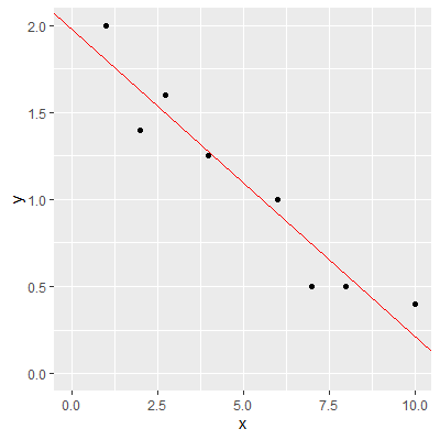
[1] -0.1766045
beta0_hat = ybar - beta1_hat*xbar
beta0_hat
[1] 1.980829
ggplot(dat, aes(x=x,y=y))+
geom_point()+
xlim(0,10)+
ylim(0,2)+
geom_abline(intercept=beta0_hat, slope=beta1_hat, color="red")
# find the fitted values of the line
yhat = beta0_hat + beta1_hat*x
#find the vertical distances of the points to the line
dists = y - yhat
#sum the vertical distances
sum(dists)
[1] -1.110223e-16
#sum the squared vertical distances
sum(dists^2)
[1] 0.2066899
Note that the sum of the vertical distances, $\sum \left(Y_i-\hat{Y}_i\right)$, is practically zero ($-1.110223e-16$).
The sum of the squared vertical distances, $\sum \left(Y_i-\hat{Y}_i\right)^2$, is $0.2066899$. Compare this to the smallest sum of squared distances you found in Table 1.3.2
Table 1.3.2
| $X$ | $Y$ | $\hat{Y}$ | $(Y-\hat{Y})$ | $(Y-\hat{Y})^2$ |
|---|---|---|---|---|
| 1 | 2 | |||
| 2 | 1.4 | |||
| 2.75 | 1.6 | |||
| 4 | 1.25 | |||
| 6 | 1 | |||
| 7 | 0.5 | |||
| 8 | 0.5 | |||
| 10 | 0.4 | |||
| Sum: |
The
[response variable] ~ [predictor variable(s)]
For our example, we will have the formula
fit = lm(y~x, data=dat)
fit


Call:
lm(formula = y ~ x, data = dat)

Coefficients:
(Intercept)            x
     1.9808      -0.1766


#to get the fitted values
fit$fitted.values


        1         2         3         4         5         6         7         8
1.8042248 1.6276203 1.4951669 1.2744112 0.9212021 0.7445976 0.5679931 0.2147840


#to get the vertical distances
fit$residuals


          1           2           3           4           5           6           7           8
 0.19577520 -0.22762027  0.10483313 -0.02441121  0.07879786 -0.24459761 -0.06799308  0.18521598


#sum of the squared distances
fit$residuals^2 %>% sum()


[1] 0.2066899