2.6 Predicting the Response

In Section 2.5, we estimated the mean of all$Y$s for some value of $X_{h}$.

Suppose we want to predict one value of the response variable $Y$ for some value of $X_{h}$. We will denote this predicted value as $Y_{h\left(pred\right)}$

Our best point predictor will be the mean (since it is the most likely value). If we knew the the true regression line, then we could predict at \begin{align*} Y_{h\left(pred\right)} & =\beta_{0}+\beta_{1}X_{h} \end{align*} The variance of $Y_{h\left(pred\right)}$ would be \begin{align*} Var\left[Y_{h}\right] & =\sigma^{2} \end{align*} Then we can be $\left(1-\alpha\right)100\%$ confident that the predicted value $Y_{h\left(pred\right)}$ is \begin{align*} z_{\alpha/2}\sigma \end{align*} units away from the line.

If we don't know $\sigma$, then we could estimate it with $s$ and we can be $\left(1-\alpha\right)100\%$ confident that the predicted value $Y_{h\left(pred\right)}$ is \begin{align*} t_{\alpha/2}s \end{align*} units away from the line.

Of course, we do not know the true regression line. We will need to estimate it first.

Using the least squares estimators, we will predict at \begin{align*} \hat{Y}_{h} & =b_{0}+b_{1}X_{h} \end{align*}

Since $\hat{Y}_{h}$ is a random variable, it will have a sampling distribution. From (2.19) , that sampling distribution has a variance of \begin{align*} Var\left[\hat{Y}_{h}\right] & =\sigma^{2}\left(\frac{1}{n}+\frac{\left(X_{h}-\bar{X}\right)^{2}}{\sum\left(X_{i}-\bar{X}\right)^{2}}\right) \end{align*} Thus, the variance of the prediction of $Y_{h\left(pred\right)}$ will be the sum of the variance of the response variable: \begin{align*} \sigma^{2} \end{align*} and the variance of the fitted line: \begin{align*} \sigma^{2}\left(\frac{1}{n}+\frac{\left(X_{h}-\bar{X}\right)^{2}}{\sum\left(X_{i}-\bar{X}\right)^{2}}\right) \end{align*} So the variance of $Y_{h\left(pre\right)}$ is \begin{align*} Var\left[Y_{h\left(pre\right)}\right] & =\sigma^{2}+\sigma^{2}\left(\frac{1}{n}+\frac{\left(X_{h}-\bar{X}\right)^{2}}{\sum\left(X_{i}-\bar{X}\right)^{2}}\right)\\ & =\sigma^{2}\left(1+\frac{1}{n}+\frac{\left(X_{h}-\bar{X}\right)^{2}}{\sum\left(X_{i}-\bar{X}\right)^{2}}\right) \end{align*}

Since $Y$ is normally distributed, then we have a $\left(100-\alpha\right)100\%$ prediction interval for $Y_{h\left(pred\right)}$ as \begin{align*} \hat{Y}_{h} & \pm t_{\alpha/2}\sqrt{s^{2}\left(1+\frac{1}{n}+\frac{\left(X_{h}-\bar{X}\right)^{2}}{\sum\left(X_{i}-\bar{X}\right)^{2}}\right)}\qquad\qquad(2.21) \end{align*}

Let's examine the trees data from Example 2.2.1.

Recall the least squares fit:

library(datasets)
library(tidyverse)


ggplot(data=trees, aes(x=Girth, y=Volume))+
  geom_point()+
  geom_smooth(method='lm',formula=y~x,se = F)

fit = lm(Volume~Girth, data=trees)
fit
Call:
lm(formula = Volume ~ Girth, data = trees)

Coefficients:
(Intercept)        Girth  
    -36.943        5.066 



#to get the correlations between all
#variables in the dataset
cor(trees)
           Girth    Height    Volume
Girth  1.0000000 0.5192801 0.9671194
Height 0.5192801 1.0000000 0.5982497
Volume 0.9671194 0.5982497 1.0000000


#get the coefficient of determination
fit %>% summary() %>% .$r.squared
[1] 0.9353199

To find the confidence and prediction intervals, we must construct a new data frame with the value of $X_h$. This value is then used, along with the lm object, to the predict function. If no value of $X_h$ is provided, then predict will provide intervals for all values of $X$ found in the data used in lm.

# get a 95% confidence interval for the mean Volume
# when girth is 16
xh=data.frame(Girth=16)

fit %>% predict(xh,interval="confidence",level=0.95)
       fit      lwr      upr
1 44.11024 42.01796 46.20252


# 95% prediction interval for one value of Volume when
# girth is 16
fit %>% predict(xh,interval="prediction",level=0.95)
       fit     lwr      upr
1 44.11024 35.1658 53.05469

We can plot the confidence interval for all values of $X$ by using the geom_smooth command in ggplot:

ggplot(data=trees, aes(x=Girth, y=Volume))+
  geom_point()+
  geom_smooth(method='lm',formula=y~x)  
                            

We can plot prediction intervals by adding them manually:

pred_int = fit %>% predict(interval="prediction",level=0.95) %>% as.data.frame()
dat = cbind(trees, pred_int)

ggplot(data=dat, aes(x=Girth, y=Volume))+
  geom_point()+
  geom_smooth(method='lm',formula=y~x)+
  geom_line(aes(y=lwr), color = "red", linetype = "dashed")+
  geom_line(aes(y=upr), color = "red", linetype = "dashed")+
  geom_smooth(method=lm, se=TRUE)

  
                            

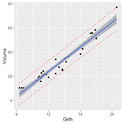
Note that the prediction interval (the red dashed lines) is wider than the confidence interval. This is because the prediction interval has the extra source of variability.