Fill in Blanks
Home
1.1 Bivariate Relationships
1.2 Probabilistic Models
1.3 Estimation of the Line
1.4 Properties of the Least Squares Estimators
1.5 Estimation of the Variance
2.1 The Normal Errors Model
2.2 Inferences for the Slope
2.3 Inferences for the Intercept
2.4 Correlation and Coefficient of Determination
2.5 Estimating the Mean Response
2.6 Predicting the Response
3.1 Residual Diagnostics
3.2 The Linearity Assumption
3.3 Homogeneity of Variance
3.4 Checking for Outliers
3.5 Correlated Error Terms
3.6 Normality of the Residuals
4.1 More Than One Predictor Variable
4.2 Estimating the Multiple Regression Model
4.3 A Primer on Matrices
4.4 The Regression Model in Matrix Terms
4.5 Least Squares and Inferences Using Matrices
4.6 ANOVA and Adjusted Coefficient of Determination
4.7 Estimation and Prediction of the Response
5.1 Multicollinearity and Its Effects
5.2 Adding a Predictor Variable
5.3 Outliers and Influential Cases
5.4 Residual Diagnostics
5.5 Remedial Measures
3.3 Homogeneity of Variance
"My philosophy is basically this, and this is something that I live by, and I always have, and I always will: Don't ever, for any reason, do anything, to anyone, for any reason, ever, no matter what, no matter where, or who, or who you are with, or where you are going, or where you've been, ever, for any reason whatsoever." - Michael Scott
As we did in Section 3.2.1, we can plot the residuals against the predictor variable $X$ or against the fitted values $\hat{Y}$ to help determine whether the variance of the error term $\varepsilon$ is constant .
When the variance is constant, we say the model hashomoscedasticity . When the variance is nonconstant, we say the model has heteroscedasticity .
When the variance is constant, we say the model has
When examining a residual plot for non-constant variance, we look for any clear changes in the spread of the residuals. One common clear pattern seen when heteroscedasticity is present is a cone pattern.
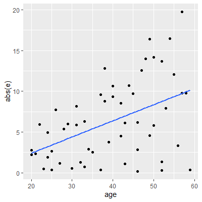
We are usually not concerned about the sign of the residual when examining for heteroscedasticity. Thus, it is common to plot theabsolute residuals or the squared residuals vs the predictor variable or fitted values.
Usually a least squares line is then fit to the absolute residual or squared residuals plot. If this line has a significant slope, then this gives evidence that the variance is nonconstant.
We are usually not concerned about the sign of the residual when examining for heteroscedasticity. Thus, it is common to plot the
Usually a least squares line is then fit to the absolute residual or squared residuals plot. If this line has a significant slope, then this gives evidence that the variance is nonconstant.
We will model the diastolic blood pressure by the age of 54 healthy adult women. The data are found in Kutner et al.
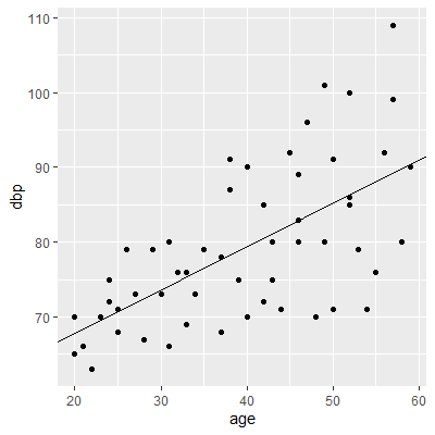
By examining the scatterplot of dbp vs age, we already see evidence of nonconstant variance.
In any of the residual plots we examine, we see the "cone" shape of the residuals which indicates the variance is nonconstant.
Kutner, M. H., Nachtsheim, C. J., Neter, J., & Li, W. (2005). Applied linear statistical models (Vol. 5). Boston: McGraw-Hill Irwin. pg 107
library(tidyverse)

dat = read.table("http://www.jpstats.org/Regression/data/bloodpressure.txt", header=T)

fit = lm(dbp~age, data=dat)

ggplot(dat, aes(x=age, y=dbp))+
  geom_point()+
  geom_abline(slope = fit$coefficients[2], intercept=fit$coefficients[1])
By examining the scatterplot of dbp vs age, we already see evidence of nonconstant variance.
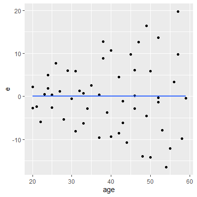
dat$e = fit %>% resid()
dat$yhat = fit %>% fitted()


#use the geom_smooth function to add a least squares line
#for the residuals, the least squares line will always be horizontal
#at 0
ggplot(dat, aes(x=age, y=e))+
  geom_point()+
  geom_smooth(method = "lm",se = F)
#plot the squared residuals and add least squares line
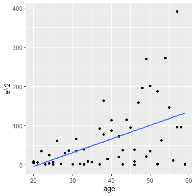
ggplot(dat, aes(x=age, y=e^2))+
geom_point()+
geom_smooth(method = "lm",se = F)
#plot the squared residuals and add least squares line
ggplot(dat, aes(x=age, y=abs(e)))+
  geom_point()+
  geom_smooth(method = "lm",se = F)
In any of the residual plots we examine, we see the "cone" shape of the residuals which indicates the variance is nonconstant.
We can set up a hypothesis test for heteroscedasticity:
\begin{align*}
H_0:&\text{ the variance is constant}\\
H_a:&\text{ the variance is non-constant}
\end{align*}
The procedures we will use usually test for variance that increases or decreases over the values of $X$. That is, the spread of the points about the line is a cone shape such as seen in Example 3.3.1.
The Levene test (Levene 1960)
Now, define the absolute deviation from the mean $$ d_{ik}=|e_{ik}-\bar{e}_{j}| $$ An ANOVA F-test is then performed on the $k$ groups. The ANOVA F-test will be discussed more in Chapter 6. A small p-value is evidence that the variance is non-constant over the values of $X$.
TheBrown-Forsythe test (Brown and Forsythe 1974)
Levene, H. 1960. “Robust Tests for Equality of Variances,”. In Contributions to Probability and Statistics, Edited by: Olkin, I. 278–92. Palo Alto, Calif.: Stanford University Press.
starts by dividing the range of the predictor variable $X$ into $k$ intervals. For each of the intervals, calculate the mean of the residuals in that interval $\bar{e}_{j}$ where $j$ denotes the $j$th interval.
Now, define the absolute deviation from the mean $$ d_{ik}=|e_{ik}-\bar{e}_{j}| $$ An ANOVA F-test is then performed on the $k$ groups. The ANOVA F-test will be discussed more in Chapter 6. A small p-value is evidence that the variance is non-constant over the values of $X$.
The
Brown, M. B., & Forsythe, A. B. (1974). Robust tests for the equality of variances. Journal of the American Statistical Association, 69(346), 364-367.
is a modification of the Levene test in which the median $\tilde{e}_k$ is used instead of the mean $\bar{e}_l$. This test is robust against nonnormal errors.
A second test for non-constant variance is the Breusch-Pagan test (Breusch and Pagan 1979)
in Example 3.3.1 shows the squared residuals plotted against $X$ and the fitted line.
If the variance is non-constant, then the slope of this line will be non-zero. Thus, a test for the slope is conducted. A small p-value is evidence that the variance is non-constant.
Because it is testing the slope, the Breusch-Pagan test assumes the error terms are independent and normally distributed.
Breusch, T. S., & Pagan, A. R. (1979). A simple test for heteroscedasticity and random coefficient variation. Econometrica: Journal of the Econometric Society, 1287-1294.
. This test assumes the variance for each $\varepsilon_i$ is related to the values of $X$ in the following way:
$$
\ln \sigma^2_i = \gamma_0 + \gamma_1 X_i
$$
Hence, a linear regression is assumed between $\sigma^2$ and $X$. We can fit the line by squaring the residuals and regressing on $X$. The third plot
If the variance is non-constant, then the slope of this line will be non-zero. Thus, a test for the slope is conducted. A small p-value is evidence that the variance is non-constant.
Because it is testing the slope, the Breusch-Pagan test assumes the error terms are independent and normally distributed.
Let's examine the data from Example 3.3.1 again.
If you want the Brown-Forsythe test, then you will need to determine the $k$ groups yourself and then use thebf.test function in onewaytests package.
In thelmtest package, the Breusch-Pagan test can be conducted by using the bptest function.
Since the p-value is low, then there is sufficient evidence to conclude the variance is not constant through different values of $X$.
If you want the Brown-Forsythe test, then you will need to determine the $k$ groups yourself and then use the
In the
library(tidyverse)
library(lmtest)

dat = read.table("http://www.jpstats.org/Regression/data/bloodpressure.txt", header=T)

fit = lm(dbp~age, data=dat)

#Breusch-Pagan test
bptest(dbp~age, data=dat)


	studentized Breusch-Pagan test

data:  dbp ~ age
BP = 12.541, df = 1, p-value = 0.0003981
Since the p-value is low, then there is sufficient evidence to conclude the variance is not constant through different values of $X$.