Fill in Blanks
Home
1.1 Bivariate Relationships
1.2 Probabilistic Models
1.3 Estimation of the Line
1.4 Properties of the Least Squares Estimators
1.5 Estimation of the Variance
2.1 The Normal Errors Model
2.2 Inferences for the Slope
2.3 Inferences for the Intercept
2.4 Correlation and Coefficient of Determination
2.5 Estimating the Mean Response
2.6 Predicting the Response
3.1 Residual Diagnostics
3.2 The Linearity Assumption
3.3 Homogeneity of Variance
3.4 Checking for Outliers
3.5 Correlated Error Terms
3.6 Normality of the Residuals
4.1 More Than One Predictor Variable
4.2 Estimating the Multiple Regression Model
4.3 A Primer on Matrices
4.4 The Regression Model in Matrix Terms
4.5 Least Squares and Inferences Using Matrices
4.6 ANOVA and Adjusted Coefficient of Determination
4.7 Estimation and Prediction of the Response
5.1 Multicollinearity and Its Effects
5.2 Adding a Predictor Variable
5.3 Outliers and Influential Cases
5.4 Residual Diagnostics
5.5 Remedial Measures
5.5 Remedial Measures
"And I knew exactly what to do. But in a much more real sense, I had no idea what to do."
- Michael Scott
We will list again the assumptions of model (4.18)
\begin{align*}
{\textbf{Y}}= & {\textbf{X}}{\boldsymbol{\beta}}+{\boldsymbol{\varepsilon}}\\
& \boldsymbol{\varepsilon} \sim N_{n}\left({\bf 0},\sigma^{2}{\bf I}\right) \qquad (4.18)
\end{align*}
and also discuss the problems violations of these assumptions present and what can be done when they are violated.
-
Linearity: Violating linearity will lead to incorrect conclusions about the relationship between $Y$ and the predictor variables and thus lead to incorrect estimations and predictions.
As discussed in Section 5.4.1, a transformation on the $X$ variables can help with linearity. -
Normality of the residuals: The t-test, F-test, confidence intervals, and prediction intervals all depend on normality of the residuals (or at least symmetric distribution).
If we do not have normality, then we cannot do the inferences for the model. A transformation on $Y$ may help with normality (or at least get to a symmetric distribution), however, we tend to lose interpretation in our inferences as discussed in Section 5.4.2.
If we cannot obtain normality through a transformation, or we wish to keep interpretation and not do a transformation, then we can still do inferences based on bootstrapping.
We first discussed bootstrapping in Section 1.4.5. We will discuss it in more detail in Section 5.5.2 below. -
Independence of the residuals: As discussed in Section 5.4.3, if there is significant autocorrelation in the residuals, then a time series model will be needed.
It was discussed at the end of Example 3.5.1 that a difference could be used to remove simple autocorrelation. The downside to doing a difference is that, once again, you lose interpretation in your inferences. -
Constant variance: Very much like the normality assumption, the constant variance assumption affects the inferences made for the model. Recall all the equations for the variance of the estimated coefficients (4.31)
\begin{align*} {\bf s}^{2}\left[{\bf b}\right] & =MSE\left({\bf X}^{\prime}{\bf X}\right)^{-1}\qquad(4.31) \end{align*}, the variance of the mean response (4.47)\begin{align*} s^{2}\left[\hat{Y}_{h}\right] & =MSE{\bf X}_{h}^{\prime}\left({\bf X}^{\prime}{\bf X}\right)^{-1}{\bf X}_{h}\qquad(4.47) \end{align*}, and the variance of the prediction (4.50)\begin{align*} s^{2}\left[Y_{h\left(pred\right)}\right] & =MSE\left(1+{\bf X}_{h}^{\prime}\left({\bf X}^{\prime}{\bf X}\right)^{-1}{\bf X}_{h}\right)\qquad(4.50) \end{align*}. Each involves MSE which is an estimate of the constant variance $\sigma^2$. If $\sigma^2$ is not constant, then MSE is not the estimator we need. We would need an estimator that takes into account the nonconstant variance.
Taking a transformation of $Y$ could help stabilize the variance, however, we would lose interpretation due to the transformation. Using a method known as weighted least squares (discussed in Section 5.5.2 below) can help with nonconstant variance. -
Uncorrelated predictor variables: In Section 5.1 we discussed the problems of having highly correlated predictor variables which is known as multicollinearity.
In Chapter 7, we will discuss model selection and hope we can select a subset of the predictor variables that do not have multicollinearity.
In some applications, it is very difficult to have a subset of predictor variables that do not have multicollinearity. When this is the case, a particular type of regression, known as ridge regression, can be used. This will be discussed in Section 5.5.4 below.
In Section 1.4.5, we bootstrapped the observations in order to estimated the sampling distributions for $\beta_0$ and $\beta_1$.
We did this due to not having any assumptions on the distribution of the error terms at that point. In Chapter 2, we started to assume that the error terms are normally distributed. Based on the normality assumption, we could determine the sampling distributions for the coefficients theoretically without need to bootstrap.
When the normality assumption does not hold, then we can use the bootstrap to estimate the sampling distributions of the coefficients and for the mean response. We could also use it for the distribution of the predicted values.
Thus, we can still obtain confidence intervals for the coefficients, confidence intervals for the mean response, and prediction intervals even when normality does not hold.
How the bootstrap works in regression is determined by the assumptions that hold for our model.
If the model is a good model for our data, the variance $\sigma^2$ is constant, and the predictor variables are regarded as fixed, then we usefixed $X$ sampling.
In fixed $X$ sampling, the regression is fitted on the sample data and the fitted values, $\hat{Y}_i$, and the residuals, $e_i$ are obtained. A bootstrap sample of size $n$ are then obtained from the residuals which are denoted $e^*_i$. The bootstrap $Y$ values are found as $$ Y^*_i = \hat{Y}_i +e^*_i\qquad(5.17) $$ These bootstrapped $Y_i^*$ are regressed on the original predictor variables. This procedure is done a large number of times and the resulting distributions of the coefficients $b^*_i$ and fitted values $\hat{Y}^*_i$ can be used as estimates of the corresponding sampling distributions.
If there is doubt in adequacy of the model, the variance $\sigma^2$ is not constant, and/or the predictor variables cannot be regarded as fixed, then we userandom $X$ sampling.
In random $X$ sampling, the observations (including $Y$ and the predictor variables) are bootstrapped and then the resulting bootstrapped sample is used to fit the model. This is what is shown in Section 1.4.5.
If the model is a good model for our data, the variance $\sigma^2$ is constant, and the predictor variables are regarded as fixed, then we use
In fixed $X$ sampling, the regression is fitted on the sample data and the fitted values, $\hat{Y}_i$, and the residuals, $e_i$ are obtained. A bootstrap sample of size $n$ are then obtained from the residuals which are denoted $e^*_i$. The bootstrap $Y$ values are found as $$ Y^*_i = \hat{Y}_i +e^*_i\qquad(5.17) $$ These bootstrapped $Y_i^*$ are regressed on the original predictor variables. This procedure is done a large number of times and the resulting distributions of the coefficients $b^*_i$ and fitted values $\hat{Y}^*_i$ can be used as estimates of the corresponding sampling distributions.
If there is doubt in adequacy of the model, the variance $\sigma^2$ is not constant, and/or the predictor variables cannot be regarded as fixed, then we use
In random $X$ sampling, the observations (including $Y$ and the predictor variables) are bootstrapped and then the resulting bootstrapped sample is used to fit the model. This is what is shown in Section 1.4.5.
We will examine the fitness dataset from the olsrr library.
In this dataset, we want to predict the oxygen level of the participants based on six predictor variables.
In this dataset, we want to predict the oxygen level of the participants based on six predictor variables.
library(tidyverse)
library(car)
library(olsrr)
library(GGally)
dat = fitness
fit = lm(oxygen~., data=dat)
#plot residual vs fitted values
ols_plot_resid_fit(fit)
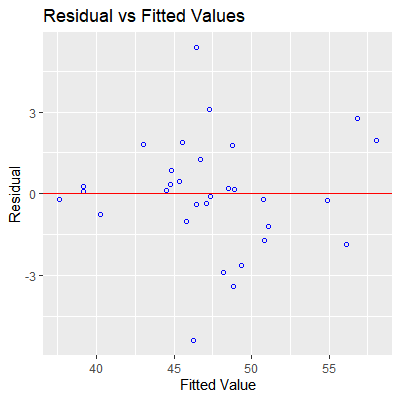
#check normality of residuals
ols_plot_resid_qq(fit)
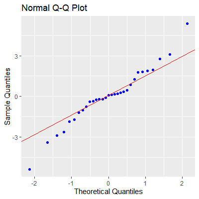
#there is some evidence against normality
######################################
#use Boot from car library
#for fixed X sampling
fit.boot = Boot(fit,method = "residual")
#examine the estimated sampling distributions
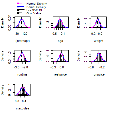
hist(fit.boot,ci = "perc")
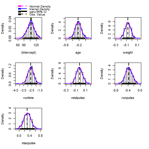
#obtain the estimated intervals by using the percentiles
Confint(fit.boot, type = "perc")
Bootstrap percent confidence intervals
Estimate 2.5 % 97.5 %
(Intercept) 102.93447948 77.97542617 127.00831140
age -0.22697380 -0.42913486 -0.02710536
weight -0.07417741 -0.17414308 0.02861982
runtime -2.62865282 -3.35725062 -1.87312652
restpulse -0.02153364 -0.14648837 0.10066258
runpulse -0.36962776 -0.59439761 -0.14316919
maxpulse 0.30321713 0.04094179 0.56322466
#if we want the CI for the mean response
fit.boot = Boot(fit,
f=function(x) predict(x),
method="residual"
)
# hist(fit.boot, ci="perc") #will give a lot of plots
ci.boot = Confint(fit.boot, level = .90,type = "perc")
ci.boot
Bootstrap percent confidence intervals
Estimate 5 % 95 %
1 44.47989 43.12460 45.82126
2 56.15193 54.40209 57.91953
3 51.07101 49.14650 53.01065
4 44.82437 42.82514 46.65981
5 40.21969 38.57365 41.85127
6 48.77620 46.93062 50.53377
7 45.77446 44.13655 47.37188
8 46.47031 44.96952 47.85776
9 46.23856 45.10592 47.26455
10 47.11347 45.34132 48.94985
11 39.15672 37.27567 40.89511
12 48.83817 47.55931 50.07698
13 44.78867 43.27731 46.17896
14 45.35278 43.50071 47.14560
15 48.49038 46.59471 50.40198
16 45.56593 44.26748 46.80740
17 48.19544 46.48934 49.89766
18 56.80409 54.82873 58.75674
19 43.01322 41.97873 44.08555
20 48.92032 47.25914 50.61772
21 58.07935 55.56178 60.85537
22 37.59931 35.24451 40.02302
23 47.36768 46.00396 48.73269
24 50.86149 48.87978 52.64878
25 49.32029 48.35797 50.29754
26 47.27381 45.34594 49.24392
27 46.46145 44.51649 48.56671
28 54.88064 53.13734 56.48647
29 39.13237 36.93808 41.53519
30 50.75065 48.50151 52.79709
31 46.67735 44.75923 48.59272
#If we want prediction intervals, we can estimate them
#by adding an estimate of the standard error to the CIs
lb = ci.boot[,2]-summary(fit)$sigma
ub = ci.boot[,3]+summary(fit)$sigma
cbind(lb, ub)
lb ub
1 40.80766 48.13821
2 52.08514 60.23648
3 46.82955 55.32759
4 40.50819 48.97676
5 36.25670 44.16822
6 44.61367 52.85072
7 41.81961 49.68883
8 42.65257 50.17471
9 42.78897 49.58150
10 43.02437 51.26680
11 34.95873 43.21205
12 45.24236 52.39392
13 40.96036 48.49591
14 41.18376 49.46255
15 44.27776 52.71892
16 41.95053 49.12435
17 44.17239 52.21461
18 52.51178 61.07368
19 39.66178 46.40250
20 44.94219 52.93467
21 53.24484 63.17232
22 32.92756 42.33997
23 43.68701 51.04964
24 46.56283 54.96572
25 46.04102 52.61449
26 43.02900 51.56087
27 42.19954 50.88366
28 50.82039 58.80341
29 34.62113 43.85214
30 46.18456 55.11404
31 42.44229 50.90967
######################################
#for random X sampling
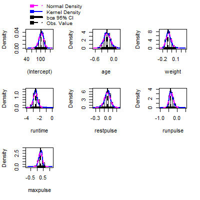
fit.boot = Boot(fit,method ="case")
hist(fit.boot,ci = "perc")
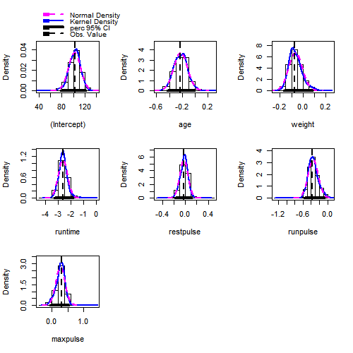
Confint(fit.boot, type = "perc")
Bootstrap percent confidence intervals
Estimate 2.5 % 97.5 %
(Intercept) 102.93447948 78.8257793 121.211569303
age -0.22697380 -0.4271126 -0.003604713
weight -0.07417741 -0.1638569 0.078350665
runtime -2.62865282 -3.2729013 -1.856616289
restpulse -0.02153364 -0.1695045 0.103453614
runpulse -0.36962776 -0.5670954 -0.084875196
maxpulse 0.30321713 -0.0389997 0.539058584
In Example 5.5.1 above, we used the percentiles of the bootstrapped sampling distributions as the lower and upper limits of the confidence intervals.
Another method that has been shown to perform better than the percentile confidence intervals is called thebias -corrected accelerated bootstrap (BCa) confidence intervals.
The details of the BCa intervals are beyond the scope of this course, but they correct by a bias factor. This factor is the proportion of the bootstrap values that are below the observed value from the original data. The skewness of the bootstrapped distribution is also taken into account.
In theConfint function in car library, we can use type="bca" argument to obtain the BCa intervals.
Another method that has been shown to perform better than the percentile confidence intervals is called the
The details of the BCa intervals are beyond the scope of this course, but they correct by a bias factor. This factor is the proportion of the bootstrap values that are below the observed value from the original data. The skewness of the bootstrapped distribution is also taken into account.
In the
We will find the BCa intervals for the fitness data from Example 5.5.1
library(tidyverse)
library(car)
library(olsrr)
library(GGally)

dat = fitness

fit = lm(oxygen~., data=dat)

######################################
#use Boot from car library
#for fixed X sampling
fit.boot = Boot(fit,method = "residual")

#examine the estimated sampling distributions
hist(fit.boot,ci="bca")


#obtain the estimated intervals by using the percentiles
Confint(fit.boot, type = "bca")

Bootstrap bca confidence intervals

                Estimate       2.5 %       97.5 %
(Intercept) 102.93447948 78.64544654 125.28707305
age          -0.22697380 -0.41256198  -0.03123658
weight       -0.07417741 -0.17733127   0.03293815
runtime      -2.62865282 -3.36959155  -1.90932155
restpulse    -0.02153364 -0.15330644   0.10262791
runpulse     -0.36962776 -0.57395998  -0.13127816
maxpulse      0.30321713  0.06901184   0.56737373


#if we want the CI for the mean response
fit.boot = Boot(fit,
                f=function(x) predict(x),
                method="residual"
)
# hist(fit.boot, ci="bca") #will give a lot of plots
ci.boot = Confint(fit.boot, level = .90,type = "bca")
ci.boot

Bootstrap bca confidence intervals

   Estimate      5 %     95 %
1  44.47989 43.19700 45.95443
2  56.15193 54.47388 58.17231
3  51.07101 49.14579 52.93122
4  44.82437 42.84039 46.74859
5  40.21969 38.54027 41.91698
6  48.77620 46.97458 50.61228
7  45.77446 44.23742 47.51168
8  46.47031 45.14926 47.83557
9  46.23856 45.22704 47.31320
10 47.11347 45.21398 49.05815
11 39.15672 37.52816 40.79624
12 48.83817 47.52348 50.05933
13 44.78867 43.45494 46.30294
14 45.35278 43.68496 47.22900
15 48.49038 46.61568 50.43589
16 45.56593 44.43070 46.86263
17 48.19544 46.51984 50.02518
18 56.80409 54.92480 58.62409
19 43.01322 41.94126 44.15988
20 48.92032 47.38658 50.80905
21 58.07935 55.67431 60.95297
22 37.59931 35.36820 40.37902
23 47.36768 45.86086 48.84815
24 50.86149 49.07262 52.92968
25 49.32029 48.33039 50.37146
26 47.27381 45.32940 49.03806
27 46.46145 44.57589 48.40999
28 54.88064 53.13659 56.71417
29 39.13237 36.84930 41.60175
30 50.75065 48.70225 52.97453
31 46.67735 44.81198 48.61059


######################################
#for random X sampling
fit.boot = Boot(fit,method ="case")
hist(fit.boot,ci = "bca")


Confint(fit.boot, type = "bca")

Bootstrap bca confidence intervals

                Estimate       2.5 %       97.5 %
(Intercept) 102.93447948 79.73553158 122.42433713
age          -0.22697380 -0.43908923   0.01138664
weight       -0.07417741 -0.17099960   0.06335917
runtime      -2.62865282 -3.45457177  -1.97806308
restpulse    -0.02153364 -0.18914034   0.09868646
runpulse     -0.36962776 -0.59172336  -0.13820186
maxpulse      0.30321713  0.01761627   0.56672408


#for the BCa intervals for the mean response
fit.boot = Boot(fit,
                f=function(x) predict(x),
                method="case"
)
# hist(fit.boot, ci="bca") #will give a lot of plots
ci.boot = Confint(fit.boot, level = .90,type = "bca")
ci.boot

Bootstrap bca confidence intervals

   Estimate      5 %     95 %
1  44.47989 36.22395 47.54938
2  56.15193 55.08704 60.83164
3  51.07101 48.82015 59.90441
4  44.82437 36.00138 47.97292
5  40.21969 35.57193 44.15655
6  48.77620 44.53464 59.73944
7  45.77446 36.88359 50.45913
8  46.47031 37.60539 54.99150
9  46.23856 37.30047 54.09247
10 47.11347 39.23819 57.61948
11 39.15672 36.15681 39.25965
12 48.83817 44.67720 59.85935
13 44.78867 35.57384 48.09630
14 45.35278 36.62762 49.57328
15 48.49038 44.09346 59.56124
16 45.56593 36.78675 49.53676
17 48.19544 43.08846 58.95941
18 56.80409 56.72094 61.10893
19 43.01322 35.31870 45.50090
20 48.92032 44.41061 59.20576
21 58.07935 58.73705 60.49549
22 37.59931 35.48381 37.01394
23 47.36768 38.78943 57.64387
24 50.86149 48.11916 61.13406
25 49.32029 45.72511 59.79763
26 47.27381 38.35916 57.41420
27 46.46145 37.30186 54.83402
28 54.88064 50.13182 60.82878
29 39.13237 36.07901 39.73133
30 50.75065 48.53119 61.28423
31 46.67735 37.90126 55.82728
Sometimes a transformation on $Y$, such as a log transformation, can help stabilize nonconstant variance. However, if the linearity assumption between $Y$ and the predictor variables seem reasonable, then transforming $Y$ may violate the linearity assumption.
If we cannot transform $Y$, we can adjust model (4.18)unbiased but they
no longer have minimum variance . That is, they are no longer the BLUEs.
To obtain unbiased estimators with minimum variance, we must take into account the different variances for the different $Y$ observations. Observations with small variances provide more reliable information about the regression function than those with large variances.
Therefore, we will want toweight the observations on the fit based on the variances of the observations.
If we cannot transform $Y$, we can adjust model (4.18)
\begin{align*}
{\textbf{Y}}= & {\textbf{X}}{\boldsymbol{\beta}}+{\boldsymbol{\varepsilon}}\\
& \boldsymbol{\varepsilon} \sim N_{n}\left({\bf 0},\sigma^{2}{\bf I}\right) \qquad (4.18)
\end{align*}
so that the variance term is allow to vary for different observations. Thus, we will have
\begin{align*}
{\textbf{Y}}= & {\textbf{X}}{\boldsymbol{\beta}}+{\boldsymbol{\varepsilon}}\\
& \boldsymbol{\varepsilon} \overset{iid}{\sim} N\left(0,\sigma_i^{2}\right) \qquad (5.18)
\end{align*}
The least squares estimators (4.21)
\begin{align*}
{\bf b}=\left({\bf X}^{\prime}{\bf X}\right)^{-1}{\bf X}^{\prime}{\bf Y}\qquad(4.21)
\end{align*}
could still be used. These estimators are To obtain unbiased estimators with minimum variance, we must take into account the different variances for the different $Y$ observations. Observations with small variances provide more reliable information about the regression function than those with large variances.
Therefore, we will want to
If the variances $\sigma_{i}^{2}$ are known, we can specify the weights
as
\begin{align*}
w_{i} & =\frac{1}{\sigma_{i}^{2}}\qquad(5.19)
\end{align*}
We can specify diagonal weight matrix as
\begin{align*}
{\bf W} & =\left[\begin{array}{cccc}
w_{1} & 0 & \cdots & 0\\
0 & w_{2} & \cdots & 0\\
\vdots & \vdots & \ddots & \vdots\\
0 & 0 & \cdots & w_{n}
\end{array}\right]\qquad(5.20)
\end{align*}
These weights can be included in the least squares estimators as
\begin{align*}
{\bf b}_{w} & =\left({\bf X}^{\prime}{\bf W}{\bf X}\right)^{-1}{\bf X}^{\prime}{\bf W}{\bf Y}\qquad(5.21)
\end{align*}
The estimated covariance matrix of the weighted least squares (wls)
estimators is
\begin{align*}
{\bf s}^{2}\left[{\bf b}_{w}\right] & =\left({\bf X}^{\prime}{\bf W}{\bf X}\right)^{-1}\qquad(5.22)
\end{align*}
Compare this to the estimated covariance matrix for the ordinary (un-weighted)
least squares (ols) estimators in (4.31)
\begin{align*}
{\bf s}^{2}\left[{\bf b}\right] & =MSE\left({\bf X}^{\prime}{\bf X}\right)^{-1}\qquad(4.31)
\end{align*}
. Instead of using MSE for
an estimate of $\sigma^{2}$, (5.22) uses the weight matrix which
takes into account how the variance changes for different observations.
For the wls estimators in (5.22)
Most of the time, the variance will vary in some systematic pattern. For example, the cone shape discussed in Example 3.3.1.
We can estimate a pattern like this by first fitting the model without any weights. We then examine the absolute values of the residuals vs the fitted values. We can regress these absolute residuals on the fitted values. This fitted model will be an estimate of the standard deviation function. Squaring these fitted values gives us an estimate of the variance function. The reciprocal of this variance function provides an estimate of the weights.
Other systematic patterns in the residual plots may require other ways to obtain an estimated variance function.
For example, if the plot of the residuals against $X_2$ suggests that the variance increases rapidly with increases in $X_2$ up to a point and then increases more slowly, then we should regress the absolute residuals against $X_2$ and $X_2^2$.
If the wls estimates differs greatly from the ols estimates, it is common to take the squared or absolute residuals from the wls fit and then re-estimate the variance function. This is done again until the changes in the estimates become small between iterations.
This is known asiteratively reweighted least squares (irls).
\begin{align*}
{\bf s}^{2}\left[{\bf b}_{w}\right] & =\left({\bf X}^{\prime}{\bf W}{\bf X}\right)^{-1}\qquad(5.22)
\end{align*}
, it is fairly straight forward if the variances $\sigma^2_i$ are known. In practice, these variances will be unknown and need to estimated.
Most of the time, the variance will vary in some systematic pattern. For example, the cone shape discussed in Example 3.3.1.
We can estimate a pattern like this by first fitting the model without any weights. We then examine the absolute values of the residuals vs the fitted values. We can regress these absolute residuals on the fitted values. This fitted model will be an estimate of the standard deviation function. Squaring these fitted values gives us an estimate of the variance function. The reciprocal of this variance function provides an estimate of the weights.
Other systematic patterns in the residual plots may require other ways to obtain an estimated variance function.
For example, if the plot of the residuals against $X_2$ suggests that the variance increases rapidly with increases in $X_2$ up to a point and then increases more slowly, then we should regress the absolute residuals against $X_2$ and $X_2^2$.
If the wls estimates differs greatly from the ols estimates, it is common to take the squared or absolute residuals from the wls fit and then re-estimate the variance function. This is done again until the changes in the estimates become small between iterations.
This is known as
We will examine the blood pressure data from Example 3.3.1.
library(tidyverse)
library(car)
library(datasets)
library(GGally)
dat = read.table("http://www.jpstats.org/Regression/data/bloodpressure.txt", header=T)
fit = lm(dbp~age, data=dat)
ols_plot_resid_fit(fit)
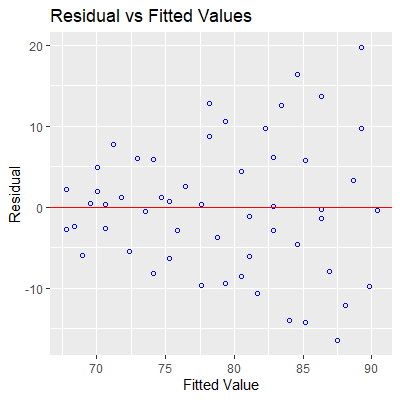
#we see evidence of nonconstant variance
#fit absolute residuals against fitted values
y = fit %>% resid() %>% abs()
x = fit %>% fitted()
fit.res = lm(y~x)
#the fitted values will be used for the weights
w = 1/(fitted.values(fit.res)^2)
#now use the weights
fit.w = lm(dbp~age, data=dat, weights = w)
# We can see the difference in the standard errors of
# the coefficients when using wls
fit %>% summary
Call:
lm(formula = dbp ~ age, data = dat)
Residuals:
Min 1Q Median 3Q Max
-16.4786 -5.7877 -0.0784 5.6117 19.7813
Coefficients:
Estimate Std. Error t value Pr(>|t|)
(Intercept) 56.15693 3.99367 14.061 2e-16 ***
age 0.58003 0.09695 5.983 2.05e-07 ***
---
Signif. codes: 0 ‘***’ 0.001 ‘**’ 0.01 ‘*’ 0.05 ‘.’ 0.1 ‘ ’ 1
Residual standard error: 8.146 on 52 degrees of freedom
Multiple R-squared: 0.4077, Adjusted R-squared: 0.3963
F-statistic: 35.79 on 1 and 52 DF, p-value: 2.05e-07
fit.w %>% summary
Call:
lm(formula = dbp ~ age, data = dat, weights = w)
Weighted Residuals:
Min 1Q Median 3Q Max
-2.0230 -0.9939 -0.0327 0.9250 2.2008
Coefficients:
Estimate Std. Error t value Pr(>|t|)
(Intercept) 55.56577 2.52092 22.042 2e-16 ***
age 0.59634 0.07924 7.526 7.19e-10 ***
---
Signif. codes: 0 ‘***’ 0.001 ‘**’ 0.01 ‘*’ 0.05 ‘.’ 0.1 ‘ ’ 1
Residual standard error: 1.213 on 52 degrees of freedom
Multiple R-squared: 0.5214, Adjusted R-squared: 0.5122
F-statistic: 56.64 on 1 and 52 DF, p-value: 7.187e-10
#let's find 95% prediction intervals for ols and wls
ci.w = predict(fit.w, interval="prediction")
ci = predict(fit, interval="prediction")
#add these to the data frame so that we can plot
dat$ols.yhat = fit %>% fitted()
dat$wls.yhat = fit.w %>% fitted()
dat$wls.lwr = ci.w[,2]
dat$wls.upr = ci.w[,3]
dat$ols.lwr = ci[,2]
dat$ols.upr = ci[,3]
ggplot(dat, aes(x=age, y=dbp))+
geom_point()+
geom_line(aes(y=ols.yhat), col="red")+
geom_line(aes(y=ols.lwr), col="red")+
geom_line(aes(y=ols.upr), col="red")+
geom_line(aes(y=wls.yhat), col="blue")+
geom_line(aes(y=wls.lwr), col="blue")+
geom_line(aes(y=wls.upr), col="blue")+
ylim(40, 120)
#note how the wls intervals allow for changing
#variability in the observations.
When there influential outliers the data which cannot be justifiably removed, then the fit will be affected by these values.
We can use the same idea from wls in which observations will have different weights when fitting the model.
When the effect of outlying cases are dampened in the fit, then it is calledrobust regression. There are many different procedures for robust regression. We will only use irls robust regression here.
There is much research into different weighting functions that should be used. We will just use the weights used in therlm function in the MASS library.
We can use the same idea from wls in which observations will have different weights when fitting the model.
When the effect of outlying cases are dampened in the fit, then it is called
There is much research into different weighting functions that should be used. We will just use the weights used in the
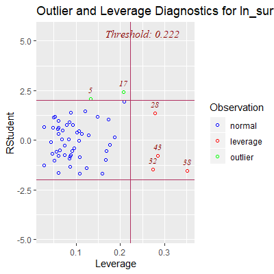
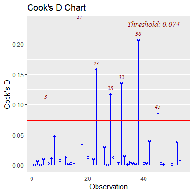
Let's examine the surgical unit data from Example 5.3.2.
library(tidyverse)
library(car)
library(olsrr)
library(MASS)

dat = read.table("http://www.jpstats.org/Regression/data/surgicalunit.txt", header=T)
dat$surv_days=NULL
dat$gender=NULL
dat$alc_heavy=NULL
dat$alc_mod=NULL

#ols fit
fit = lm(ln_surv_days~., data=dat)

#examine outliers and infuence
ols_plot_resid_lev(fit)
ols_plot_cooksd_chart(fit)


#irls robust regression
fit.irls = rlm(ln_surv_days~., data=dat)

#examine the change in the coefficients
summary(fit.irls)

Call: rlm(formula = ln_surv_days ~ ., data = dat)
Residuals:
      Min        1Q    Median        3Q       Max
-0.404338 -0.172208 -0.002364  0.176442  0.550496

Coefficients:
            Value   Std. Error t value
(Intercept)  3.9748  0.3141    12.6538
blood_clot   0.0899  0.0307     2.9317
prog_ind     0.0131  0.0024     5.3851
enzyme_test  0.0166  0.0022     7.4214
liver_test   0.0055  0.0561     0.0984
age         -0.0037  0.0034    -1.0964

Residual standard error: 0.2622 on 48 degrees of freedom

summary(fit)

Call:
lm(formula = ln_surv_days ~ ., data = dat)

Residuals:
     Min       1Q   Median       3Q      Max
-0.38972 -0.18936  0.00492  0.17813  0.51173

Coefficients:
             Estimate Std. Error t value Pr(>|t|)
(Intercept)  4.047377   0.296662  13.643   2e-16 ***
blood_clot   0.090811   0.028959   3.136  0.00292 **
prog_ind     0.012969   0.002300   5.638 8.91e-07 ***
enzyme_test  0.016130   0.002107   7.655 7.33e-10 ***
liver_test   0.011042   0.053012   0.208  0.83587
age         -0.004579   0.003196  -1.433  0.15842
---
Signif. codes:  0 ‘***’ 0.001 ‘**’ 0.01 ‘*’ 0.05 ‘.’ 0.1 ‘ ’ 1

Residual standard error: 0.2482 on 48 degrees of freedom
Multiple R-squared:  0.7691,	Adjusted R-squared:  0.745
F-statistic: 31.97 on 5 and 48 DF,  p-value: 3.462e-14
We have seen in Section 5.1 that multicollinearity causes the least
squares estimates to be imprecise.
If we allow some bias in our estimators, then we can have estimators that are more precise. This is due to the relationship \begin{align*} E\left[\left(\hat{\beta}-\beta\right)^{2}\right] & =Var\left[\hat{\beta}\right]+\left(E\left[\hat{\beta}\right]-\beta\right)^{2} \end{align*}Ridge regression starts by transforming the variables as
\begin{align*}
Y_{i}^{*} & =\frac{1}{\sqrt{n-1}}\left(\frac{Y_{i}-\overline{Y}}{s_{Y}}\right)\\
X_{ik}^{*} & =\frac{1}{\sqrt{n-1}}\left(\frac{X_{ik}-\overline{X}_{k}}{s_{k}}\right)\qquad(5.23)
\end{align*}
This is known as the correlation transformation .
The estimates are then found bypenalizing the least squares criterion
\begin{align*}
Q & =\sum\left[Y_{i}^{*}-\left(b_{1}^{*}X_{i1}^{*}+\cdots+b_{p-1}^{*}X_{i,p-1}^{*}\right)\right]^{2}+\lambda\left[\sum_{j=1}^{p-1}\left(b_{j}^{*}\right)^{2}\right]\qquad(5.24)
\end{align*}
The added term gives a penalty for large coefficients. Thus, the estimators
are biased toward 0. Because of this, the ridge estimators are called
shrinkage estimators.
There are a number of methods for determining $\lambda$ which are beyond the scope of our class. In R, we will use thecv.glmnet function
from the glmnet library which uses a process known as cross validation.
The ridge estimators are more stable than the ols estimators, however, the distributional properties of these estimators are not easily found. Therefore, bootstrapping would be needed to find confidence intervals or prediction interval.
If we allow some bias in our estimators, then we can have estimators that are more precise. This is due to the relationship \begin{align*} E\left[\left(\hat{\beta}-\beta\right)^{2}\right] & =Var\left[\hat{\beta}\right]+\left(E\left[\hat{\beta}\right]-\beta\right)^{2} \end{align*}
The estimates are then found by
There are a number of methods for determining $\lambda$ which are beyond the scope of our class. In R, we will use the
The ridge estimators are more stable than the ols estimators, however, the distributional properties of these estimators are not easily found. Therefore, bootstrapping would be needed to find confidence intervals or prediction interval.
library(tidyverse)
library(car)
library(olsrr)
library(MASS)
library(glmnet)
dat = read.table("http://www.jpstats.org/Regression/data/BodyFat.txt", header=T)
#ols fit
fit = lm(bfat~., data=dat)
vif(fit)
tri thigh midarm
708.8429 564.3434 104.6060
#clear evidence of multicollinearity
#for cv.glmnet, you must input the variables as matrices
X = dat[,1:3] %>% as.matrix()
y = dat[,4] %>% as.matrix()
#must specify alpha=0 for ridge regression
fit.ridge = cv.glmnet(X, y, alpha=0)
#plot the mean square error for different lambdas
plot(fit.ridge)
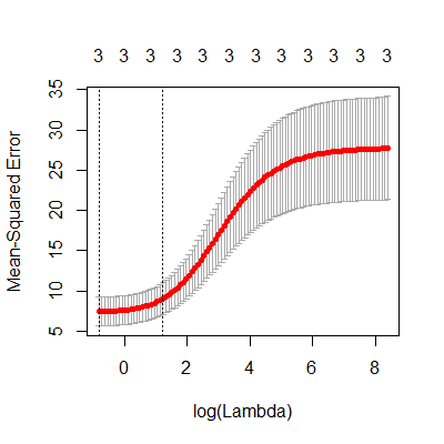
#by default, cv.glmnet chooses the range of lambda for you
#we see in the plot above that the minimum mean square error
#is at the smallest lambda. This is shown by the dotted
#vertical line. The other vertical line is one std dev away
#form the minimum mean square error.
#We will want to see if there
#are smaller lambdas we can try
lambdas = 10^seq(-4, 4, by = .1)
fit.ridge = cv.glmnet(X, y, alpha=0,lambda = lambdas)
plot(fit.ridge)
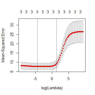
#now we see minimum mean squared error
#we can obtain the ridge estimates by
b.ridge = predict(fit.ridge, s ="lambda.min", type = "coefficients")
b.ridge
4 x 1 sparse Matrix of class "dgCMatrix"
1
(Intercept) -9.7998760
tri 0.4201644
thigh 0.4350961
midarm -0.1050418
#compare to ols
fit
Call:
lm(formula = bfat ~ ., data = dat)
Coefficients:
(Intercept) tri thigh midarm
117.085 4.334 -2.857 -2.186