2.3 Inferences for the Intercept

"I think Comic Sans always screams FUN."
- Jerry Gergich (Parks and Recreation)

2.3.1 Interpretation of the Intercept

The interpretation for the intercept $\beta_0$ in model (2.1)

\begin{align*} Y_i=&\beta_0+\beta_1X_i+\varepsilon_i\\ \varepsilon_i\overset{iid}{\sim}& N\left(0,\sigma^2\right)\qquad\qquad\qquad\qquad(2.1) \end{align*}

may not be useful for many applications.

In Sections 2.5 and 2.6, we will discuss how to use the model for estimation and prediction. In these inferences, the estimation or prediction should only be made in the range of the values of $X$. This is because the information we have is only on that range. Therefore, we should only make inferences on what we have information for.

In Figure 2.3.1, a scatterplot of engine displacement vs mile per gallon (mpg) are shown for 32 vehicles. This data is the mtcars dataset in the datasets library.

Suppose the red points in the plot are the only observations we have. We fit model (2.1)

\begin{align*} Y_i=&\beta_0+\beta_1X_i+\varepsilon_i\\ \varepsilon_i\overset{iid}{\sim}& N\left(0,\sigma^2\right)\qquad\qquad\qquad\qquad(2.1) \end{align*}

to only those red points. The blue line is the resulting least squares line.

Figure 2.3.1: Scatterplot of mtcars data

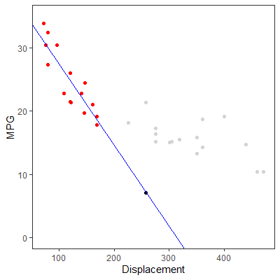Now suppose we use the fitted model to predict the mpg of a vehicle with an engine with a displacement of 258. The black point on the line at $X=258$ is the predicted mpg of 7.079638. Clearly, this value of displacement is beyond any displacement that we used to fit the model.

Consider the gray points as observations that we did not have to fit the model. Note how the regression line does not model those gray points very well. In fact, our prediction of 7.079638 mpg is far below an actual observation of an engine with displacement of 159 which had a mpg of 21.4.

This example shows that we should not use the model outside the range of the values of $X$. To do so is called extrapolating and forces us to make assumptions about the relationship between $X$ and $Y$ that we have no information for.

We should also avoid making an interpretation of the intercept if the range of $X$ does not contain zero. So we should only interpret $\beta_0$ as the mean value of $Y$ when $X=0$ if zero is in the range of $X$.

2.3.2 Sampling Distribution for $b_0$

The BLUE for $\beta_{0}$ is the least squares estimator $b_0$.

In Section 1.4.2 and Section 1.4.3 we discussed that the mean of the sampling distribution of $b_{0}$ is $$ E[b_0]=\beta_0 $$ with a variance of \begin{align*} Var\left[b_{0}\right] & =\sigma^{2}\left[\frac{1}{n}+\frac{\left(\bar{X}\right)^{2}}{\sum \left(X_{i}-\bar{X}\right)^{2}}\right]\qquad\qquad\qquad(1.15) \end{align*}

As we did with $b_1$, we will assume the normal errors model (2.1)

\begin{align*} Y_i=&\beta_0+\beta_1X_i+\varepsilon_i\\ \varepsilon_i\overset{iid}{\sim}& N\left(0,\sigma^2\right)\qquad\qquad\qquad\qquad(2.1) \end{align*}

and examine the sampling distribution.

Recall that we can write $b_{0}$ as \begin{align*} b_{0} & =\sum c_{i}Y_{i}\qquad\qquad\qquad(1.6) \end{align*} where \begin{align*} c_{i} & =\frac{1}{n}-\bar{X}k_{i} \end{align*} which shows that $b_{0}$ is a linear combination of $Y$.

Since $Y$ is normally distributed by (2.2)

\begin{align*} Y_i{\sim} N\left(\beta_0+\beta_1X_i,\sigma^2\right)\qquad\qquad\qquad(2.2) \end{align*}

, then we can apply Theorem 2.1

\begin{align*} Y_i=&\beta_0+\beta_1X_i+\varepsilon_i\\ \varepsilon_i\overset{iid}{\sim}& N\left(0,\sigma^2\right)\qquad\qquad\qquad\qquad(2.1) \end{align*}

which implies that $b_{0}$ is normally distributed. That is, \begin{align*} b_{0} & \sim N\left(\beta_{0},\sigma^2\left[\frac{1}{n}+\frac{\left(\bar{X}\right)^2}{\sum \left(X_i - \bar{X}\right)^2}\right]\right)\quad\quad\quad(2.7) \end{align*}

Standardized Score

Since $b_{0}$ is normally distributed, we can standardize it so that the resulting statistic will have a standard normal distribution.

Therefore, we have \begin{align*} z=\frac{b_{0}-\beta_{0}}{\sqrt{\sigma^2\left[\frac{1}{n}+\frac{\left(\bar{X}\right)^2}{\sum \left(X_i - \bar{X}\right)^2}\right]}} & \sim N\left(0,1\right)\qquad\qquad\qquad(2.8) \end{align*}

Studentized Score

As we did with $b_1$ in Section 2.2.2, we can studentized $b_0$ to obtain \begin{align*} t & =\frac{b_{0}-\beta_{0}}{\sqrt{s^2\left[\frac{1}{n}+\frac{\left(\bar{X}\right)^2}{\sum \left(X_i - \bar{X}\right)^2}\right]}} \end{align*}

2.3.3 Confidence Interval for $\beta_0$

Using the $t$ statistic above, a $\left(1-\alpha\right)100$% confidence interval for $\beta_{0}$ is \begin{align*} b_{0}\pm t_{\alpha/2}\sqrt{s^2\left[\frac{1}{n}+\frac{\left(\bar{X}\right)^2}{\sum \left(X_i - \bar{X}\right)^2}\right]}\qquad\qquad\qquad(2.9) \end{align*}

2.3.4 Hypothesis Tests for $\beta_0$

We can test the hypotheses \begin{align*} H_{0}: & \beta_{0}=\beta_{0}^{0}\\ H_{a}: & \beta_{0}\ne\beta_{0}^{0} \end{align*} where $\beta_{0}^{0}$ is the hypothesized value.

We can test this hypothesis with the $t$ test statistic assuming the null hypothesis is true: \begin{align*} t= & \frac{b_{0}-\beta_{0}^{0}}{\sqrt{s^2\left[\frac{1}{n}+\frac{\left(\bar{X}\right)^2}{\sum \left(X_i - \bar{X}\right)^2}\right]}}\qquad\qquad\qquad(2.10) \end{align*}

In Example 2.2.1, we showed how to do a confidence interval and hypothesis test for $\beta_1$. The R code also provided a confidence interval and hypothesis test for $\beta_0$. Note that the hypothesis test was testing the hypothesis $H_a:\beta_0=0$.

« 2.2: Inferences for the Slope 2.4: Correlation and Coefficient of Determination »