3.4 Checking for Outliers

"If the statistics are boring, then you've got the wrong numbers." - Edward Tufte

3.4.1 Outliers With Respect to $X$ and $Y$

When checking for outliers, we must think in terms of two dimensions since we have two variables, $X$ and $Y$.

Since we are interested in modeling the response variable $Y$ in model (2.1)

\begin{align*} Y_i=&\beta_0+\beta_1X_i+\varepsilon_i\\ \varepsilon_i\overset{iid}{\sim}& N\left(0,\sigma^2\right)\qquad\qquad\qquad\qquad(2.1) \end{align*}

, we will mainly be concerned outliers with respect to $Y$. However, outliers with respect to $X$ may also be of concern if it affects the fitted line.

Effect on the Fitted Line

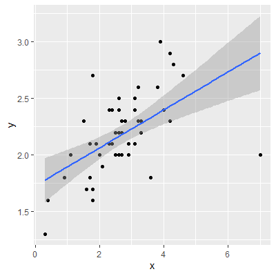
To show how outliers can effect the fitted line, 50 observations are shown in Figure 3.4.1 along with the fitted line shown in blue.

You can click on the points and move them on the plot and see the effect on the fitted line.

Try moving a point in the $X$ direction and then try moving in the $Y$ direction.

Note that if the point is moved away from the blue line closer to the ends (such at around $X=0$ or $X=6$) it has more of an effect on the fitted line than moving a point away from the line around the middle (such at around $X=3$).

Figure 3.4.1: Outiers

3.4.2 Detecting Outliers with Semistudentized Residual Plots

Since the effect on the fitted line is determined mainly by how far the point is from the line, we will identify outliers by examining the residuals, in particular, the semistudentized residuals \begin{align*} e_{i}^{*} & =\frac{e_{i}-\bar{e}}{\sqrt{MSE}}\\ & =\frac{e_{i}}{\sqrt{MSE}}\qquad\qquad\qquad(3.3) \end{align*} We can plot $e_{i}^{*}$ against $X$ or against $\hat{Y}$. A general rule of thumb is any value of $e_{i}^{*}$ below -4 or above 4 should be considered an outlier. Note that this rule is only applicable to large $n$.

In Chapter 5, we will discuss other methods for detecting outliers.

Example 3.4.1

Let's examine 50 observations of $X$ and $Y$:

library(tidyverse)

dat = read.table("http://www.jpstats.org/Regression/data/example_03_04_01.csv", header=T, sep=",")

ggplot(dat, aes(x=x,y=y))+
  geom_point()+
  geom_smooth(method = "lm")

                             

fit = lm(y~x, data=dat)

#calculate semistudentized residuals
dat$e.star = fit$residuals / summary(fit)$sigma

ggplot(dat, aes(x=x, y=e.star))+
  geom_point()

We can see from the semistudentized plot that there is one observation with a value of $e^*$ below -3. Although this is not below the rule of thumb of -4, we note that our sample size $n$ is only moderate and not large. So we may want to investigate an observation with a value of $e^*$ below -3.

Once we see there is a potential outlier, we must investigate why it is an outlier. If the observation is unusually small or large due to a data recording error, then perhaps the value can be corrected or just deleted from the dataset. If we cannot determine this is the cause of the outlier for certain, then we should not remove the observation. This observation could be unusual just due to chance.

« 3.3: Homogeneity of Variance 3.5: Correlated Error Terms »