Fill in Blanks
Home
1.1 Bivariate Relationships
1.2 Probabilistic Models
1.3 Estimation of the Line
1.4 Properties of the Least Squares Estimators
1.5 Estimation of the Variance
2.1 The Normal Errors Model
2.2 Inferences for the Slope
2.3 Inferences for the Intercept
2.4 Correlation and Coefficient of Determination
2.5 Estimating the Mean Response
2.6 Predicting the Response
3.1 Residual Diagnostics
3.2 The Linearity Assumption
3.3 Homogeneity of Variance
3.4 Checking for Outliers
3.5 Correlated Error Terms
3.6 Normality of the Residuals
4.1 More Than One Predictor Variable
4.2 Estimating the Multiple Regression Model
4.3 A Primer on Matrices
4.4 The Regression Model in Matrix Terms
4.5 Least Squares and Inferences Using Matrices
4.6 ANOVA and Adjusted Coefficient of Determination
4.7 Estimation and Prediction of the Response
5.1 Multicollinearity and Its Effects
5.2 Adding a Predictor Variable
5.3 Outliers and Influential Cases
5.4 Residual Diagnostics
5.5 Remedial Measures
2.2 Inferences for the Slope
"If you do not know how to ask the right question, you discover nothing."
- W. E. Demining
With model (2.1)
Recall that $\beta_1$ is the populationslope . Recall from algebra that the slope is the change in $Y$ for a unit increase of $X$.
If $Y$increases as $X$ increases, then the slope is positive. If it decreases as $X$ increases, then the slope is negative.
In model (2.1)mean of $Y$ for a unit increase in $X$. This is because the line represents the mean of the response ($Y$) for a given value of $X$.
\begin{align*}
Y_i=&\beta_0+\beta_1X_i+\varepsilon_i\\
\varepsilon_i\overset{iid}{\sim}& N\left(0,\sigma^2\right)\qquad\qquad\qquad\qquad(2.1)
\end{align*}
, we can make inferences on the parameters $\beta_0$ and $\beta_1$. In this section, we will focus on inferences for $\beta_1$. In Section 2.3, we will discuss inferences for $\beta_0$.
Recall that $\beta_1$ is the population
If $Y$
In model (2.1)
\begin{align*}
Y_i=&\beta_0+\beta_1X_i+\varepsilon_i\\
\varepsilon_i\overset{iid}{\sim}& N\left(0,\sigma^2\right)\qquad\qquad\qquad\qquad(2.1)
\end{align*}
, the slope represents a change in the
If the slope is zero, then this means the mean of $Y$ does not change as $X$ increases. In other words, the line would just be a horizontal line.
For example, in Figure 2.2.1, 200 observations from the model $$ \begin{align*} Y_i & = 0X_i + \varepsilon_i\\ \varepsilon_i & \overset{iid}{\sim}N(0,1) \end{align*} $$ are shown.
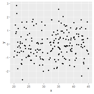 The slope in the model is in fact zero. Note from the scatterplot that the line that would best represent the relationship between $X$ and $Y$ is a horizontal line. That is, the mean of $Y$ does not appear to change as $X$ changes.
If $Y$ does not change as $X$ increases, then using $X$ to predict $Y$ in the linear model (2.1)
Thus, one of our first inferences should be for the population slope $\beta_1$.
For example, in Figure 2.2.1, 200 observations from the model $$ \begin{align*} Y_i & = 0X_i + \varepsilon_i\\ \varepsilon_i & \overset{iid}{\sim}N(0,1) \end{align*} $$ are shown.
Figure 2.2.1: Scatterplot for zero slope model
If $Y$ does not change as $X$ increases, then using $X$ to predict $Y$ in the linear model (2.1)
\begin{align*}
Y_i=&\beta_0+\beta_1X_i+\varepsilon_i\\
\varepsilon_i\overset{iid}{\sim}& N\left(0,\sigma^2\right)\qquad\qquad\qquad\qquad(2.1)
\end{align*}
is not useful.
Thus, one of our first inferences should be for the population slope $\beta_1$.
We discussed in Section 1.4.4 that the least squared estimator $b_{1}$
is the BLUE for $\beta_{1}$.
We also discussed in Section 1.4.2 and Section 1.4.3 that the mean of the sampling distribution of $b_{1}$ is $$ E[b_1]=\beta_1 $$ with a variance of \begin{align*} Var\left[b_{1}\right] & =\frac{\sigma^{2}}{\sum \left(X_{i}-\bar{X}\right)^{2}}\qquad\qquad\qquad(1.14) \end{align*}
We used bootstrapping in Section 1.4.5 to estimate the shape of the sampling distribution. Now with the normal errors model (2.1)
Recall that we can write $b_{1}$ as \begin{align*} b_{1} & =\sum k_{i}Y_{i}\qquad\qquad\qquad(1.5) \end{align*} where \begin{align*} k_{i} & =\frac{X_{i}-\bar{X}}{\sum \left(X_{i}-\bar{X}\right)^{2}} \end{align*} which shows that $b_{1}$ is alinear combination of $Y$.
Since $Y$ is normally distributed by (2.2)
We also discussed in Section 1.4.2 and Section 1.4.3 that the mean of the sampling distribution of $b_{1}$ is $$ E[b_1]=\beta_1 $$ with a variance of \begin{align*} Var\left[b_{1}\right] & =\frac{\sigma^{2}}{\sum \left(X_{i}-\bar{X}\right)^{2}}\qquad\qquad\qquad(1.14) \end{align*}
We used bootstrapping in Section 1.4.5 to estimate the shape of the sampling distribution. Now with the normal errors model (2.1)
\begin{align*}
Y_i=&\beta_0+\beta_1X_i+\varepsilon_i\\
\varepsilon_i\overset{iid}{\sim}& N\left(0,\sigma^2\right)\qquad\qquad\qquad\qquad(2.1)
\end{align*}
, we
can know the shape of the sampling distribution without having to
estimate it.
Recall that we can write $b_{1}$ as \begin{align*} b_{1} & =\sum k_{i}Y_{i}\qquad\qquad\qquad(1.5) \end{align*} where \begin{align*} k_{i} & =\frac{X_{i}-\bar{X}}{\sum \left(X_{i}-\bar{X}\right)^{2}} \end{align*} which shows that $b_{1}$ is a
Since $Y$ is normally distributed by (2.2)
\begin{align*}
Y_i{\sim} N\left(\beta_0+\beta_1X_i,\sigma^2\right)\qquad\qquad\qquad(2.2)
\end{align*}
, then we can apply Theorem 2.1
Theorem 2.1 Sum of Independent Normal Random Variables:
If $$ X_i\sim N\left(\mu_i,\sigma_i^2\right) $$ are independent, then the linear combination $\sum_i a_iX_i$ is also normally distributed where $a_i$ are constants. In particular $$ \sum_i a_iX_i \sim N\left(\sum_i a_i\mu_i, \sum_i a_i^2\sigma_i^2\right) $$
which
implies that $b_{1}$ is normally distributed. That is,
\begin{align*}
b_{1} & \sim N\left(\beta_{1},\frac{\sigma^{2}}{\sum\left(X_{i}-\bar{X}\right)^{2}}\right)\quad\quad\quad(2.3)
\end{align*}
If $$ X_i\sim N\left(\mu_i,\sigma_i^2\right) $$ are independent, then the linear combination $\sum_i a_iX_i$ is also normally distributed where $a_i$ are constants. In particular $$ \sum_i a_iX_i \sim N\left(\sum_i a_i\mu_i, \sum_i a_i^2\sigma_i^2\right) $$
Since $b_{1}$ is normally distributed, we can standardize it so that
the resulting statistic will have a standard normal distribution.
Therefore, we have \begin{align*} z=\frac{b_{1}-\beta_{1}}{\sqrt{\frac{\sigma^{2}}{\sum\left(X_{i}-\bar{X}\right)^{2}}}} & \sim N\left(0,1\right)\qquad\qquad\qquad(2.4) \end{align*}
Therefore, we have \begin{align*} z=\frac{b_{1}-\beta_{1}}{\sqrt{\frac{\sigma^{2}}{\sum\left(X_{i}-\bar{X}\right)^{2}}}} & \sim N\left(0,1\right)\qquad\qquad\qquad(2.4) \end{align*}
In practice, the standardized score $z$ is not useful since we do
not know the value of $\sigma^{2}$. In Section 1.5, we estimated
$\sigma^{2}$ with the statistic
$$
s^2 = \frac{SSE}{n-2}\qquad\qquad\qquad(1.17)
$$
It is important to note the following theorem from math stats presented here without proof:
Theorem 2.3 Distribution of the sample variance of the residuals:
For the sample variance of the residuals $s^{2}$, the quantity \begin{align*} \frac{\left(n-2\right)s^{2}}{\sigma^{2}} & =\frac{SSE}{\sigma^{2}} \end{align*} is distributed as a chi-square distribution with $n-2$ degrees of freedom. That is, \begin{align*} \frac{SSE}{\sigma^{2}} & \sim\chi^{2}\left(n-2\right) \end{align*}
We will use another important theorem form math stats (again presented without proof):
Theorem 2.4 Ratio of independent standard normal and chi-square statistics:
If $Z\sim N\left(0,1\right)$ and $W\sim\chi^{2}\left(\nu\right)$, and $Z$ and $W$ are independent, then the statistic \begin{align*} \frac{Z}{\sqrt{\frac{W}{\nu}}} \end{align*} is distributed as a Student's $t$ distribution with $\nu$ degrees of freedom.
We will take the standardized score in (2.4) and divide by \begin{align*} \sqrt{\frac{\frac{\left(n-2\right)s^{2}}{\sigma^{2}}}{\left(n-2\right)}} & =\sqrt{\frac{s^{2}}{\sigma^{2}}} \end{align*} to give us \begin{align*} t & =\frac{\frac{b_{1}-\beta_{1}}{\sqrt{\frac{\sigma^{2}}{\sum\left(X_{i}-\overline{X}\right)^{2}}}}}{\sqrt{\frac{s^{2}}{\sigma^{2}}}}\\ & =\frac{b_{1}-\beta_{1}}{\sqrt{\frac{\sigma^{2}}{\sum\left(X_{i}-\overline{X}\right)^{2}}}\sqrt{\frac{s^{2}}{\sigma^{2}}}}\\ & =\frac{b_{1}-\beta_{1}}{\sqrt{\frac{s^{2}}{\sum\left(X_{i}-\overline{X}\right)^{2}}}} \end{align*} which will have a Student's $t$ distribution with $n-2$ degrees of freedom.
We call this $t$ statistic, thestudentized score.
It is important to note the following theorem from math stats presented here without proof:
Theorem 2.3 Distribution of the sample variance of the residuals:
For the sample variance of the residuals $s^{2}$, the quantity \begin{align*} \frac{\left(n-2\right)s^{2}}{\sigma^{2}} & =\frac{SSE}{\sigma^{2}} \end{align*} is distributed as a chi-square distribution with $n-2$ degrees of freedom. That is, \begin{align*} \frac{SSE}{\sigma^{2}} & \sim\chi^{2}\left(n-2\right) \end{align*}
We will use another important theorem form math stats (again presented without proof):
Theorem 2.4 Ratio of independent standard normal and chi-square statistics:
If $Z\sim N\left(0,1\right)$ and $W\sim\chi^{2}\left(\nu\right)$, and $Z$ and $W$ are independent, then the statistic \begin{align*} \frac{Z}{\sqrt{\frac{W}{\nu}}} \end{align*} is distributed as a Student's $t$ distribution with $\nu$ degrees of freedom.
We will take the standardized score in (2.4) and divide by \begin{align*} \sqrt{\frac{\frac{\left(n-2\right)s^{2}}{\sigma^{2}}}{\left(n-2\right)}} & =\sqrt{\frac{s^{2}}{\sigma^{2}}} \end{align*} to give us \begin{align*} t & =\frac{\frac{b_{1}-\beta_{1}}{\sqrt{\frac{\sigma^{2}}{\sum\left(X_{i}-\overline{X}\right)^{2}}}}}{\sqrt{\frac{s^{2}}{\sigma^{2}}}}\\ & =\frac{b_{1}-\beta_{1}}{\sqrt{\frac{\sigma^{2}}{\sum\left(X_{i}-\overline{X}\right)^{2}}}\sqrt{\frac{s^{2}}{\sigma^{2}}}}\\ & =\frac{b_{1}-\beta_{1}}{\sqrt{\frac{s^{2}}{\sum\left(X_{i}-\overline{X}\right)^{2}}}} \end{align*} which will have a Student's $t$ distribution with $n-2$ degrees of freedom.
We call this $t$ statistic, the
We now introduce some notation for the quantile of a distribution
using the $t$ distribution for an example. The notation
\begin{align*}
t_{\alpha}
\end{align*}
represents the $1-\alpha$ quantile of the Student's $t$ distribution.
That is
\begin{align*}
P\left(T\lt t_{\alpha}\right) & =1-\alpha
\end{align*}
Using the $t$ statistic above, we can specify the middle $\left(1-\alpha\right)$ of the distribution of $t$ and have \begin{align*} -t_{\alpha/2}\lt \frac{b_{1}-\beta_{1}}{\sqrt{\frac{s^{2}}{\sum\left(X_{i}-\overline{X}\right)^{2}}}}\lt t_{\alpha/2} \end{align*} Solving this for $\beta_{1}$ gives us \begin{align*} b_{1}\pm t_{\alpha/2}\sqrt{\frac{s^{2}}{\sum\left(X_{i}-\overline{X}\right)^{2}}}\qquad\qquad\qquad(2.5) \end{align*} which is a $\left(1-\alpha\right)100$% confidence interval for $\beta_{1}$.
Using the $t$ statistic above, we can specify the middle $\left(1-\alpha\right)$ of the distribution of $t$ and have \begin{align*} -t_{\alpha/2}\lt \frac{b_{1}-\beta_{1}}{\sqrt{\frac{s^{2}}{\sum\left(X_{i}-\overline{X}\right)^{2}}}}\lt t_{\alpha/2} \end{align*} Solving this for $\beta_{1}$ gives us \begin{align*} b_{1}\pm t_{\alpha/2}\sqrt{\frac{s^{2}}{\sum\left(X_{i}-\overline{X}\right)^{2}}}\qquad\qquad\qquad(2.5) \end{align*} which is a $\left(1-\alpha\right)100$% confidence interval for $\beta_{1}$.
We can also test a hypothesis for $\beta_{1}$ such as testing if
$\beta_{1}\ne0$ since a slope of zero would indicate that the mean
of $Y$ does not change for changes in $X$.
In general, the hypotheses are \begin{align*} H_{0}: & \beta_{1}=\beta_{1}^{0}\\ H_{a}: & \beta_{1}\ne\beta_{1}^{0} \end{align*} where $\beta_{1}^{0}$ is the hypothesized value.
We can test this hypothesis with the $t$ test statistic assuming the null hypothesis is true: \begin{align*} t= & \frac{b_{1}-\beta_{1}^{0}}{\sqrt{\frac{s^{2}}{\sum\left(X_{i}-\overline{X}\right)^{2}}}}\qquad\qquad\qquad(2.6) \end{align*}
In R, a packaged called datasets include a number of available datasets. One of the datasets is called trees :
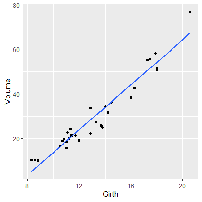
There are 31 total observations in this dataset. Variables measured are the Girth (actually the diameter measured at 54 in. off the ground), the Height, and the Volume of timber from each black cherry tree.
Suppose we want to predict Volume from Girth. We start by plotting the scatterplot.
We fit the regression model usinglm as before. We then use the summary function:
From the output, we can find the value of $b_1$ under Coefficients on the line with Girth (since Girth was the $X$ variable). The Std. Error value is the denominator of the $t$ statistic. The t value is the value of the test statistic for the hypothesis $$ H_0:\beta_1=0\\ H_a:\beta_1\ne 0 $$ The p-value for the test is listed next. In this case, the p-value is very small indicating strong evidence that $\beta_1\ne 0$.
To obtain a confidence interval for $\beta_1$, we can use theconfint function:
Thus, a 95% confidence interval for $\beta_1$ is (4.56, 5.57).
library(datasets)
head(trees)


  Girth Height Volume
1   8.3     70   10.3
2   8.6     65   10.3
3   8.8     63   10.2
4  10.5     72   16.4
5  10.7     81   18.8
6  10.8     83   19.7
There are 31 total observations in this dataset. Variables measured are the Girth (actually the diameter measured at 54 in. off the ground), the Height, and the Volume of timber from each black cherry tree.
Suppose we want to predict Volume from Girth. We start by plotting the scatterplot.
library(tidyverse)

#Note that geom_smooth is a quick way to
#add the regression line to the plot
ggplot(data=trees, aes(x=Girth, y=Volume))+
  geom_point()+
  geom_smooth(method='lm',formula=y~x,se = F)
We fit the regression model using
fit = lm(Volume~Girth, data=trees)
fit %>% summary()


Call:
lm(formula = Volume ~ Girth, data = trees)

Residuals:
   Min     1Q Median     3Q    Max
-8.065 -3.107  0.152  3.495  9.587

Coefficients:
            Estimate Std. Error t value Pr(>|t|)
(Intercept) -36.9435     3.3651  -10.98 7.62e-12 ***
Girth         5.0659     0.2474   20.48  < 2e-16 ***
---
Signif. codes:  0 ‘***’ 0.001 ‘**’ 0.01 ‘*’ 0.05 ‘.’ 0.1 ‘ ’ 1

Residual standard error: 4.252 on 29 degrees of freedom
Multiple R-squared:  0.9353,	Adjusted R-squared:  0.9331
F-statistic: 419.4 on 1 and 29 DF,  p-value: < 2.2e-16
From the output, we can find the value of $b_1$ under Coefficients on the line with Girth (since Girth was the $X$ variable). The Std. Error value is the denominator of the $t$ statistic. The t value is the value of the test statistic for the hypothesis $$ H_0:\beta_1=0\\ H_a:\beta_1\ne 0 $$ The p-value for the test is listed next. In this case, the p-value is very small indicating strong evidence that $\beta_1\ne 0$.
To obtain a confidence interval for $\beta_1$, we can use the
fit %>% confint(level = .95)


                 2.5 %     97.5 %
(Intercept) -43.825953 -30.060965
Girth         4.559914   5.571799
Thus, a 95% confidence interval for $\beta_1$ is (4.56, 5.57).