4.6 ANOVA and Adjusted Coefficient of Determination

Recall from Figure 2.4.2 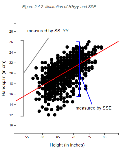in Section 2.4.3 that we used $SS_{YY}$ to denote the variability of the response variable $Y$ from its mean $\bar Y$ (without regard to the model involving $X$).

Another name for $SS_{YY}$ is the sum of squares total (SSTO). We call it this since it gives us a measure of total variability in $Y$.

In multiple regression, SSTO is still the same as $SS_{YY}$ in (2.12) . In matrix notation this can be expressed as \begin{align*} SSTO & ={\bf Y}^{\prime}{\bf Y}-\left(\frac{1}{n}\right){\bf Y}^{\prime}{\bf J}{\bf Y}\qquad(4.34) \end{align*}

Also recall from Figure 2.4.2 , the variability of $Y$ about the regression line (in simple linear regression) was expressed by SSE in (1.16) . We can think of this as the variability of $Y$ remaining after exampling some of the variability with the regression model.

In multiple regression, SSE is still the sum of the square distances between the response $Y$ and the fitted model $\hat{Y}$. Now, the fitted model is the fitted hyperplane instead of a line.

The SSE can be expressed in matrix terms as \begin{align*} SSE & =\left({\bf Y}-{\bf X}{\bf b}\right)^{\prime}\left({\bf Y}-{\bf X}{\bf b}\right)\\ & ={\bf Y}^{\prime}{\bf Y}-{\bf b}^{\prime}{\bf X}^{\prime}{\bf Y}\qquad\qquad\left(4.35\right) \end{align*}

If SSTO is the total variability of $Y$ (without of regard to the predictor variables), and SSE is the variability of $Y$ left over after explaining the variability of $Y$ with the model (including the predictor variables), we might want to know the variability of $Y$ explained by the model.

We call the variability explained by the regression model the sum of squares regression (SSR).

We will show below that SSR can be expressed as \begin{align*} SSR & =\sum\left(\hat{Y}_{i}-\bar{Y}\right)^{2}\qquad(4.36) \end{align*} which can be expressed in matrix terms as \begin{align*} SSR & ={\bf b}^{\prime}{\bf X}^{\prime}{\bf Y}-\left(\frac{1}{n}\right){\bf Y}^{\prime}{\bf J}{\bf Y}\qquad(4.37) \end{align*}

To see how SSTO, SSR, and SSE relate to each other, consider how SSTO is a sum of squares of $Y$ from its mean $\bar{Y}$: \begin{align*} Y_{i}-\bar{Y} \end{align*} We can add and subtract the fitted value $\hat{Y}_{i}$ to get \begin{align*} Y_{i}-\bar{Y} & =Y_{i}-\hat{Y}_{i}+\hat{Y}_{i}-\bar{Y}\\ & =\left(Y_{i}-\hat{Y}_{i}\right)+\left(\hat{Y}_{i}-\bar{Y}\right) \end{align*} Squaring both sides gives us \begin{align*} \left(Y_{i}-\bar{Y}\right)^{2} & =\left[\left(Y_{i}-\hat{Y}_{i}\right)+\left(\hat{Y}_{i}-\bar{Y}\right)\right]^{2}\\ & =\left(Y_{i}-\hat{Y}_{i}\right)^{2}+\left(\hat{Y}_{i}-\bar{Y}\right)^{2}+2\left(Y_{i}-\hat{Y}_{i}\right)\left(\hat{Y}_{i}-\bar{Y}\right) \end{align*} Summing both sides gives us \begin{align*} \sum\left(Y_{i}-\bar{Y}\right)^{2} & =\sum\left(Y_{i}-\hat{Y}_{i}\right)^{2}+\sum\left(\hat{Y}_{i}-\bar{Y}\right)^{2}+2\sum\left(Y_{i}-\hat{Y}_{i}\right)\left(\hat{Y}_{i}-\bar{Y}\right)\\ & =\sum\left(Y_{i}-\hat{Y}_{i}\right)^{2}+\sum\left(\hat{Y}_{i}-\bar{Y}\right)^{2}+2\sum\hat{Y}_{i}e_{i}-2\bar{Y}\sum e_{i} \end{align*} Note that $\sum\hat{Y}_{i}e_{i}=0$ from (1.22) and $\sum e_{i}=0$ from (1.20) . Therefore, we have \begin{align*} \sum\left(Y_{i}-\bar{Y}\right)^{2} & =\sum\left(\hat{Y}_{i}-\bar{Y}\right)^{2}+\sum\left(Y_{i}-\hat{Y}_{i}\right)^{2}\\ SSTO & =SSR+SSE \qquad\qquad\qquad\qquad\qquad(4.38) \end{align*} We call this the decomposition of SSTO.

The degrees of freedom can be decomposed as well. Note that the degrees of freedom for SSTO is \begin{align*} df_{SSTO} & =n-1 \end{align*} since the mean of $Y$ is needed to be estimated with $\bar{Y}$. The degrees of freedom for SSE is \begin{align*} df_{SSE} & =n-p \end{align*} since the $p$ coefficients $\beta_{0},\ldots,\beta_{p-1}$ need to be estimated with $b_{0},\ldots,b_{p-1}.$ For SSR, the degrees of freedom is \begin{align*} df_{SSR} & =p-1 \end{align*} since there are $p$ estimated coefficients $b_{0},\ldots,b_{p-1}$ but need to estimate the mean of $Y$ with $\bar{Y}$. Decomposing the degrees of freedom give us \begin{align*} n-1 & =p-1+n-p\\ df_{SSTO} & =df_{SSR}+df_{SSE}\qquad(4.29) \end{align*}

The sums of squares and degrees of freedom are commonly displayed in an analysis of variance (ANOVA) table:

Source	df	SS	MS	F	p-value
Regression	$df_{SSR}$	$SSR$
Error	$df_{SSE}$	$SSE$
Total	$df_{SSTO}$	$SSTO$

Recall from Section 3.1.1 that if we divide SSE by its degrees of freedom, we obtain the mean square error: \begin{align*} MSE & =\frac{SSE}{n-p}\qquad(4.40) \end{align*} Likewise, if we divide SSR by its degrees of freedom, we obtain the mean square regression: \begin{align*} MSR & =\frac{SSR}{p-1}\qquad(4.41) \end{align*} These values are also included in the ANOVA table:

Source	df	SS	MS	F	p-value
Regression	$df_{SSR}$	$SSR$	$MSR$
Error	$df_{SSE}$	$SSE$	$MSE$
Total	$df_{SSTO}$	$SSTO$

Note that although the sum of squares and degrees of freedom decompose, the mean squares do not. That is \begin{align*} \frac{SSTO}{n-1} & \ne MSR+MSE \end{align*} In fact, the mean square for the total ($SSTO/n-1$) does not usually show up on the ANOVA table.

In Section 2.2.4, we tested the slope in simple regression to see if there is a significant linear relationship between $X$ and $Y$.

In multiple regression, we will want to see if there is any significant linear relationship between any of the $X$s and $Y$. Thus, we want to test the hypotheses \begin{align*} H_{0}: & \beta_{1}=\beta_{2}=\cdots=\beta_{p-1}=0\\ H_{a}: & \text{at least one } \beta \text{ is not equal to zero} \end{align*} To construct a test statistic, we first note that \begin{align*} \frac{SSE}{\sigma^{2}} & \sim\chi^{2}\left(n-p\right) \end{align*} Also, if $H_{0}$ is true, then \begin{align*} \frac{SSR}{\sigma^{2}} & \sim\chi^{2}\left(p-1\right) \end{align*} The ratio of two independent chi-square random variables divided by their degrees of freedom give a statistic that follows a F-distribution.

Since $SSE/\sigma^{2}$ and $SSR/\sigma^{2}$ are independent (proof not give here), then under $H_{0}$, we can construct a test statistic as \begin{align*} F^{*} & =\left(\frac{\frac{SSR}{\sigma^{2}}}{p-1}\right)\div\left(\frac{\frac{SSE}{\sigma^{2}}}{n-p}\right)\\ & =\left(\frac{SSR}{p-1}\right)\div\left(\frac{SSE}{n-p}\right)\\ & =\frac{MSR}{MSE}\qquad\qquad\qquad\qquad(4.42) \end{align*} Large values of $F^{*}$ indicate evidence for $H_{a}$.

The test statistic and p-value are the last two components of the ANOVA table:

Source	df	SS	MS	F	p-value
Regression	$df_{SSR}$	$SSR$	$MSR$	$F^*$	$P\left(Z\ge Z^*\right)$
Error	$df_{SSE}$	$SSE$	$MSE$
Total	$df_{SSTO}$	$SSTO$

As was the case with the simple regression model, the coefficient of determination for the multiple regression model (or the coefficient of multiple determination) is \begin{align*} R^{2} & =\frac{SSR}{SSTO}\\ & =1-\frac{SSE}{SSTO}\qquad(4.43) \end{align*} The interpretation is still the same: it gives the proportion of the variation in $Y$ explained by the model using the predictor variables.

It is of importance to note that $R^{2}$ cannot decrease when adding another $X$ to the model. It can either increase (if the new $X$ explains more of the variability of $Y$) or stay the same (if the new $X$ does not explain more of the variability of $Y$). This can be seen in (4.43) by noting that SSE cannot become larger by including more $X$ variables and SSTO stays the same regardless of which $X$ variables are used.

Because of this, $R^{2}$ cannot be used for comparing the fit of models with different subsets of the $X$ variables.

A modified version of the $R^{2}$ could be used that adjusts for the number of $X$ variables. It is called the adjusted coefficient of determination denoted as $R_{a}^{2}$.

In $R_{a}^{2}$, SSE and SSTO are divided by their respective degrees of freedom: \begin{align*} R_{a}^{2} & =1-\frac{\frac{SSE}{n-p}}{\frac{SSTO}{n-1}}\\ & =1-\left(\frac{n-1}{n-p}\right)\frac{SSE}{SSTO}\qquad(4.44) \end{align*} The value of $R_{a}^{2}$ can decrease when another $X$ is included in the model because any decrease in SSE may be more than offset by the loss of a degree of freedom of SSE ($n-p$).

Let's look at the bodyfat data from Example 4.5.1.

library(tidyverse)

dat = read.table("http://www.jpstats.org/Regression/data/BodyFat.txt", header=T)

fit = lm(bfat~tri+thigh+midarm, data=dat)

# we can get the multiple R^2 and adjusted R^2 from the summary
fit %>% summary

Call:
lm(formula = bfat ~ tri + thigh + midarm, data = dat)

Residuals:
    Min      1Q  Median      3Q     Max 
-3.7263 -1.6111  0.3923  1.4656  4.1277 

Coefficients:
            Estimate Std. Error t value Pr(>|t|)
(Intercept)  117.085     99.782   1.173    0.258
tri            4.334      3.016   1.437    0.170
thigh         -2.857      2.582  -1.106    0.285
midarm        -2.186      1.595  -1.370    0.190

Residual standard error: 2.48 on 16 degrees of freedom
Multiple R-squared:  0.8014,	Adjusted R-squared:  0.7641 
F-statistic: 21.52 on 3 and 16 DF,  p-value: 7.343e-06

# to get them individually
summary(fit)$r.squared

[1] 0.8013586

summary(fit)$adj.r.squared

[1] 0.7641133


# The F test statistic and p-value can also be found from summary
summary(fit)

Call:
lm(formula = bfat ~ tri + thigh + midarm, data = dat)

Residuals:
    Min      1Q  Median      3Q     Max 
-3.7263 -1.6111  0.3923  1.4656  4.1277 

Coefficients:
            Estimate Std. Error t value Pr(>|t|)
(Intercept)  117.085     99.782   1.173    0.258
tri            4.334      3.016   1.437    0.170
thigh         -2.857      2.582  -1.106    0.285
midarm        -2.186      1.595  -1.370    0.190

Residual standard error: 2.48 on 16 degrees of freedom
Multiple R-squared:  0.8014,	Adjusted R-squared:  0.7641 
F-statistic: 21.52 on 3 and 16 DF,  p-value: 7.343e-06


#you can obtain a version of the anova table:
anova(fit)

Analysis of Variance Table

Response: bfat
          Df Sum Sq Mean Sq F value    Pr(>F)    
tri        1 352.27  352.27 57.2768 1.131e-06 ***
thigh      1  33.17   33.17  5.3931   0.03373 *  
midarm     1  11.55   11.55  1.8773   0.18956    
Residuals 16  98.40    6.15                      
---
Signif. codes:  0 ‘***’ 0.001 ‘**’ 0.01 ‘*’ 0.05 ‘.’ 0.1 ‘ ’ 1

#note that the Df, sum Sq, Mean Sq, and F test are split among the 
#X variables