3.2 The Linearity Assumption

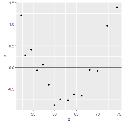
We can check the linearity assumption by plotting the residuals vs the predictor variable or plotting the residuals vs the fitted values.

We usually examine a scatterplot to determine if a linear relationship between $X$ and $Y$ is appropriate. There are times when the scatterplot makes it difficult to see if a nonlinear relationship exists. This may be the case if the observed $Y$ are close to the fitted line $\hat{Y}_i$. This usually means the slope is steep.

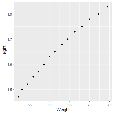
In this example, we will consider the weights (in kg) and heights (in m) of 16 women ages 30-39. The dataset is from kaggle.

library(tidyverse)

#read in data from website
dat = read_csv("http://www.jpstats.org/Regression/data/Weight_Height.csv",)

#plot the data
ggplot(dat, aes(x=Weight, y=Height))+
  geom_point()
                            

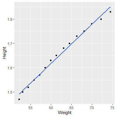
#fit the model
fit = lm(Weight~Height, data=dat)

#plot with regression line
ggplot(dat, aes(x=Weight, y=Height))+
  geom_point()+
  geom_smooth(method="lm", formula=y~x, se=F)

                            

#make dataset with Weight, the fitted values, and residuals
dat2 = tibble(x = dat$Weight, yhat = fit$fitted.values, e = fit$residuals)


#plot x by residuals
ggplot(dat2, aes(x=x, y=e))+
  geom_point()+
  geom_hline(yintercept = 0, col="red")
                            

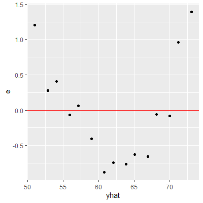
#plot fitted values by residuals
ggplot(dat2, aes(x=yhat, y=e))+
  geom_point()+
  geom_hline(yintercept = 0, col="red")

                            

Plotting the residuals against $X$ will provide the same information as plotting the residuals against $\hat{Y}$ for the simple linear regression model.

When more predictor variables are considered (Chapter 4), then plotting against the $X$ variables and plotting against $\hat{Y}$ may provide different information. It is usually helpful to plot both in that case.

When the linearity assumption does not hold (as seen in the residual plots), then a nonlinear model may be considered or a transformation on either $X$ or $Y$ can be attempted to make the relationship linear.

Transforming the response variable $Y$ may lead to issues with other assumptions such as the constant variance assumption or the normality of $\varepsilon$ assumption.

If our only concern is the linearity assumption, then transforming $X$ will be the best option. This transformation may be a square root transformation $\sqrt{X}$, a log transformation $\log{X}$, or some power transformation $X^{p}$ were $p$ is some real number.

Sometimes a transformation of $X$ will not be enough to satisfy the linearity assumption. In that case, model (2.1) should be abandoned in favor of a nonlinear model.