Fill in Blanks
Home
1.1 Bivariate Relationships
1.2 Probabilistic Models
1.3 Estimation of the Line
1.4 Properties of the Least Squares Estimators
1.5 Estimation of the Variance
2.1 The Normal Errors Model
2.2 Inferences for the Slope
2.3 Inferences for the Intercept
2.4 Correlation and Coefficient of Determination
2.5 Estimating the Mean Response
2.6 Predicting the Response
3.1 Residual Diagnostics
3.2 The Linearity Assumption
3.3 Homogeneity of Variance
3.4 Checking for Outliers
3.5 Correlated Error Terms
3.6 Normality of the Residuals
4.1 More Than One Predictor Variable
4.2 Estimating the Multiple Regression Model
4.3 A Primer on Matrices
4.4 The Regression Model in Matrix Terms
4.5 Least Squares and Inferences Using Matrices
4.6 ANOVA and Adjusted Coefficient of Determination
4.7 Estimation and Prediction of the Response
5.1 Multicollinearity and Its Effects
5.2 Adding a Predictor Variable
5.3 Outliers and Influential Cases
5.4 Residual Diagnostics
5.5 Remedial Measures
1.2 Probabilistic Models
"Math is the logic of certainty; statistics is the logic of uncertainty." - Joe Blitzstein
In Figure 1.1.3
 , four types of bivariate relationships were shown. In those cases, the relationships told us how $Y$ changes, in general, as $X$ changes.
If the relationship told us the exact value of $Y$ for a value of $X$, then the relationship would be adeterministic relationship since we can determine the value of $Y$ just by the value of $X$.
Figure 1.1.3
would then look like the figure below:
If the relationship told us the exact value of $Y$ for a value of $X$, then the relationship would be a
Figure 1.1.3
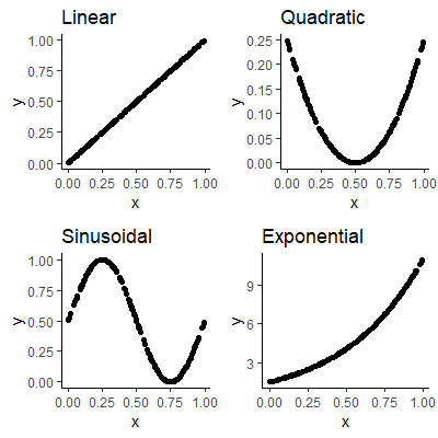
Figure 1.2.1: Deterministic Relationships
In Figure 1.1.3
, at any value of $X$ the value of $Y$ could be a range of values, however, the $Y$ values do follow the relationship, in general, as $X$ changes.
In Figure 1.2.1, the value of $Y$ must be the relationship evaluated at the value of $X$. Of course, this requires us to know what form the relationship takes.
The form of the relationship will be afunction which we will denote as
$$
Y=g(X)
$$
For those in Figure 1.2.1, the functions are : $$ \begin{align*} \text{Linear: } & g\left(X\right)=X\\ \text{Quadratic: } & g\left(X\right)=(X-0.5)^{2}\\ \text{Sinusoidal: } & g\left(X\right)=0.5\sin(2\pi X)+0.5\\ \text{Exponential: } & g\left(X\right)=1.5\exp(2X) \end{align*} $$
In Figure 1.2.1, the value of $Y$ must be the relationship evaluated at the value of $X$. Of course, this requires us to know what form the relationship takes.
The form of the relationship will be a
For those in Figure 1.2.1, the functions are : $$ \begin{align*} \text{Linear: } & g\left(X\right)=X\\ \text{Quadratic: } & g\left(X\right)=(X-0.5)^{2}\\ \text{Sinusoidal: } & g\left(X\right)=0.5\sin(2\pi X)+0.5\\ \text{Exponential: } & g\left(X\right)=1.5\exp(2X) \end{align*} $$
Deterministic relationships present us with two issues:
- We need to what what type of relationship there is between $X$ and $Y$. That is, what is $g(x)$? We can always look at a scatterplot to determine the general form of $g(X)$, but what exactly is the formula for the function? We will discuss how to estimate $g(X)$ in Sec 1.3.
- In real world data, the relationship between $X$ and $Y$ are almost never deterministic. For the handspan example, do we expect everyone who is 72 inches tall to have the exact same handspan? Clearly not. There are other factors that may help determine handspan such as gender, genetics, or other variables that are important but we do not have. Handspan could also vary due to random phenomena. Thus, we will need something more than just a deterministic model.
Let's look at the linear deterministic relationship where $g(X)=0.5+1.2X$ for some values of $X$. The scatterplot is shown in Figure 1.2.2 to the right.
If the relationship between $X$ and $Y$ isnon-deterministic , then we can express the relationship as the deterministic component, $g(X)$, plus a term representing some random error .
If the relationship between $X$ and $Y$ is
Thus, we can express the non-deterministic relationship with the model
$$
Y=g(X)+\text{random error}
$$
or, for this example,
$$
Y=0.5+1.2X+\text{random error}
$$
In the scatterplot, the random error is expressed as thevertical distance between the point and the line that represents the deterministic component (the line in this linear example).
We can express the deterministic component in the plot with a line and then each point will have some vertical distance from the line. This is represented in the model by the random error. On the scatterplot, the gray lines represent the random error.
In the scatterplot, the random error is expressed as the
We can express the deterministic component in the plot with a line and then each point will have some vertical distance from the line. This is represented in the model by the random error. On the scatterplot, the gray lines represent the random error.
Figure 1.2.2: Linear scatterplot
When we have a model that includes random error, we call the model a probabilistic model .
The model above, $$ Y=\color{red}{g(X)}+\color{gray}{\text{random error}} $$ gives us a representation of each value of $Y$. Each value will be the function $g(X)$ evaluated at $X$ plus some random error.
In the example in Figure 1.2.2, $g(X)$ was in the form of a line. It could also be any other relationship. For the remainder of this chapter, we will only focus on models that have a linear form of $g(X)$.
Thus far, we have been loose with our notation in the model. We will next introduce a formal notation for the model in Subsection 1.2.3.
The $Y$ variable is called the response , or dependent variable.
The $X$ variable is called thepredictor , explanatory , or independent variable. We will mostly refer to it as the predictor variable.
When we obtain sample data, we will use a subscript to indicate the values for each observation (ortrial ). For example, $(X_1, Y_1)$ represents the values of $X$ and $Y$ for the first trial, $(X_2, Y_2)$ for the second trial, etc.
In general, $(X_i, Y_i)$ represents the values for the $i$th trial.
The $X$ variable is called the
When we obtain sample data, we will use a subscript to indicate the values for each observation (or
In general, $(X_i, Y_i)$ represents the values for the $i$th trial.
The first model we present is called "simple " because it only has one predictor variable ($X$). It is called "linear " because the deterministic component takes the form of a line:
$$
Y_i=\beta_0+\beta_1X_i+\varepsilon_i\qquad\qquad\qquad(1.1)
$$
where:
$Y_i$ is the value of the response variable for the $i$th trial,
$\beta_0$ is aparameter representing the y-intercept of the line,
$\beta_1$ is aparameter representing the slope of the line,
$X_i$ is the value of the predictor variable for the $i$th trial,
$\varepsilon_i$ represents the random error term.
$Y_i$ is the value of the response variable for the $i$th trial,
$\beta_0$ is a
$\beta_1$ is a
$X_i$ is the value of the predictor variable for the $i$th trial,
$\varepsilon_i$ represents the random error term.
We already stated that model (1.1) is "simple" because there is only one predictor variable.
Model (1.1) is "linear in the parameters " because every parameter is only to the first power and is not multiplied or divided by another parameter.
Model (1.1) is also "linear in the predictor variable " because $X$ appears only with an exponent of one (instead of $X^2$, $X^{1/2}$, etc.).
A "linear model" means it is linear in the parameters (not necessarily linear in the predictor variables). A model that is linear in both the parameters and the predictor variables is called afirst-order model .
Model (1.1) is "
Model (1.1) is also "
A "linear model" means it is linear in the parameters (not necessarily linear in the predictor variables). A model that is linear in both the parameters and the predictor variables is called a
Since $\varepsilon_i$ represents the random error, it is random variable.
Since it is a random variable, it has a probability distribution. We will not specify the distribution yet, but will make some assumptions about it.
1. The mean of the distribution of $\varepsilon_{i}$ is 0. That is, \begin{align*} E\left[\varepsilon_{i}\right] & =0 \end{align*} Some of the points will be above the line, as in Figure 1.2.2, and some will be below the line. Those above the line will have an error with a positive value and those below the line will have an error with a negative value. If these values are averaged, the negative values will cancel out the positive values so that the mean is zero.
2. The variance of the distribution is finite and is the same for all $i$. That is, \begin{align*} Var\left[\varepsilon_{i}\right] & =\sigma^{2} \end{align*} In Figure 1.2.2, this implies the spread of the points are about the same over the entire line.
3. Any pair of error terms are uncorrelated
Recall that an informal definition of a random variable is a variable whose possible values are numerical outcomes of a random phenomenon. In other words, it is something that gives us a numeric value that we do not know precisely until we observe the data from the experiment or observational study.
Since it is a random variable, it has a probability distribution. We will not specify the distribution yet, but will make some assumptions about it.
1. The mean of the distribution of $\varepsilon_{i}$ is 0. That is, \begin{align*} E\left[\varepsilon_{i}\right] & =0 \end{align*} Some of the points will be above the line, as in Figure 1.2.2, and some will be below the line. Those above the line will have an error with a positive value and those below the line will have an error with a negative value. If these values are averaged, the negative values will cancel out the positive values so that the mean is zero.
2. The variance of the distribution is finite and is the same for all $i$. That is, \begin{align*} Var\left[\varepsilon_{i}\right] & =\sigma^{2} \end{align*} In Figure 1.2.2, this implies the spread of the points are about the same over the entire line.
3. Any pair of error terms are uncorrelated
If two random variables are uncorrelated, then they have a covariance that is 0. Recall that the covariance is a measure of how two random variables vary together. It is defined as
$$
Cov\left[X,Y\right] = E\left[\left(X-\mu_X\right)\left(Y-\mu_Y\right)\right]
$$
. That is,
\begin{align*}
Cov\left[\varepsilon_{i},\varepsilon_{j}\right]=0 & \text{ for all }i,j;i\ne j
\end{align*}
Since $Y_i$ is expressed as a function of the random variable $\varepsilon_i$ in model (1.1) random variable .
Since $Y_i$ is a random variable, then it will have a probability distribution. The mean of $Y_i$ is \begin{align*} E\left[Y_{i}\right] & =\underbrace{E\left[\beta_{0}+\beta_{1}X_{i}+\varepsilon_{i}\right]}_{E \text{ can be distributed}}\\ &\\ & =\underbrace{E\left[\beta_{0}\right]}_{\beta_0 \text{ is a constant}}+\underbrace{E\left[\beta_{1}X_{i}\right]}_{\beta_1 \text{ and }X_1\text{ are both constants}}+\underbrace{E\left[\varepsilon_{i}\right]}_{=0\text{ from the assumptions about }\varepsilon}\\\\ & =\beta_{0}+\beta_{1}X_{i}+0\\ & =\beta_{0}+\beta_{1}X_{i} \end{align*} Thus, the mean of all the $Y$ values for a given value of $X$ is just the line evaluated at $X$.
The variance of $Y_i$ is \begin{align*} Var\left[Y_{i}\right] & =\underbrace{Var\left[\beta_{0}+\beta_{1}X_{i}+\varepsilon_{i}\right]}_{\beta_{0},\beta_{1},\text{ and }X_{i}\text{ are all constants}}\\ \\ & =\underbrace{Var\left[\varepsilon_{i}\right]}_{\text{From the assumptions about }\varepsilon_{i}}\\ \\ & =\sigma^{2} \end{align*}
Since we assume the error terms are uncorrelated, then any two $Y_i$ and $Y_j$ areuncorrelated for $i,j;i\ne j$.
Although the values of $Y_i$ are random variables, we assume the values $X_i$ of the predictor variable are knownconstants .
In adesigned experiment , the design should include trials for predetermined values of $X$. For example, if you were to design an experiment where the response variable ($Y$) is reaction time for people to some stimulus after given some drug and the predictor variable ($X$) is the weight of the person, then a well designed experiment will sample subjects from predetermined weights. This will allow you to have observations for as many values of $X$ as you would like.
Frequently, one does not obtain the data in regression analysis through a designed experiment. Instead, the data comes from anobservational study . In this case, the values of $X$ do come from a random variable, however, in regression analysis, we assume the values of $X$ are observed or fixed values of the random variable.
$$
Y_i=\beta_0+\beta_1X_i+\varepsilon_i\qquad\qquad\qquad(1.1)
$$
, then $Y_i$ is also a Since $Y_i$ is a random variable, then it will have a probability distribution. The mean of $Y_i$ is \begin{align*} E\left[Y_{i}\right] & =\underbrace{E\left[\beta_{0}+\beta_{1}X_{i}+\varepsilon_{i}\right]}_{E \text{ can be distributed}}\\ &\\ & =\underbrace{E\left[\beta_{0}\right]}_{\beta_0 \text{ is a constant}}+\underbrace{E\left[\beta_{1}X_{i}\right]}_{\beta_1 \text{ and }X_1\text{ are both constants}}+\underbrace{E\left[\varepsilon_{i}\right]}_{=0\text{ from the assumptions about }\varepsilon}\\\\ & =\beta_{0}+\beta_{1}X_{i}+0\\ & =\beta_{0}+\beta_{1}X_{i} \end{align*} Thus, the mean of all the $Y$ values for a given value of $X$ is just the line evaluated at $X$.
The variance of $Y_i$ is \begin{align*} Var\left[Y_{i}\right] & =\underbrace{Var\left[\beta_{0}+\beta_{1}X_{i}+\varepsilon_{i}\right]}_{\beta_{0},\beta_{1},\text{ and }X_{i}\text{ are all constants}}\\ \\ & =\underbrace{Var\left[\varepsilon_{i}\right]}_{\text{From the assumptions about }\varepsilon_{i}}\\ \\ & =\sigma^{2} \end{align*}
Since we assume the error terms are uncorrelated, then any two $Y_i$ and $Y_j$ are
Although the values of $Y_i$ are random variables, we assume the values $X_i$ of the predictor variable are known
In a
Frequently, one does not obtain the data in regression analysis through a designed experiment. Instead, the data comes from an
We can visualize the assumptions listed above by picturing a distribution of possible values of $Y$ for each possible value of $X$.
In Figure 1.2.3, the model from Figure 1.2.2, $$ Y_i=0.5+1.2X_i+\varepsilon_i $$ is shown with ten observed values. These observations were randomly simulated from the model.
If you hover your mouse over the plot, you will see a colored vertical line to represent the distribution of values of $Y$ for the value of $X$. The darker the line, the more likely the values are.
Note that we did not specify the type of distribution for $\varepsilon$ above in our assumptions. In Figure 1.2.3, we are assuming some genericunimodal and symmetric distribution.
As you hover over the plot, notice that the distribution is the same for all values of $X$ except for the center of the distribution. The mean of the distribution will be at the line evaluated at $X$. The variability of the distribution stays the same for all values of $X$.
Based on the distribution of $Y$'s for each value of $X$, you can see how likely the observed data (the points) are in terms of the distribution. Values further (in vertical distance) from the line are less likely than those close to the line.
In the next section, we discuss how to estimate the line given some observed values.
In Figure 1.2.3, the model from Figure 1.2.2, $$ Y_i=0.5+1.2X_i+\varepsilon_i $$ is shown with ten observed values. These observations were randomly simulated from the model.
If you hover your mouse over the plot, you will see a colored vertical line to represent the distribution of values of $Y$ for the value of $X$. The darker the line, the more likely the values are.
Note that we did not specify the type of distribution for $\varepsilon$ above in our assumptions. In Figure 1.2.3, we are assuming some generic
As you hover over the plot, notice that the distribution is the same for all values of $X$ except for the center of the distribution. The mean of the distribution will be at the line evaluated at $X$. The variability of the distribution stays the same for all values of $X$.
Based on the distribution of $Y$'s for each value of $X$, you can see how likely the observed data (the points) are in terms of the distribution. Values further (in vertical distance) from the line are less likely than those close to the line.
Figure 1.2.3: Linear scatterplot