1.1 Bivariate Relationships
"Relationships? We don't need no stinking relationships!" -Michael Scott
When examining one set of data, we usually want to describe it using some basic statistics such as the mean $$\bar{Y} = \frac{1}{n}\sum_{i=1}^n Y_i $$ and the standard deviation $$ s = \sqrt{\frac{1}{n-1}\sum_{i=1}^n \left(Y_i-\bar{Y}\right)^2} $$
Recall that $\bar{Y}$ is a measure of
That is, we have a measure of where the "center" of the data tends to locate and a measure of how "spread out" is the data.
We also will want to visualize the data with a plot such as a
Suppose we have a sample of size $n=834$ of college students and we record their right handspan (in cm).
Since there is only one variable, the scatterplot will only show the data at it relates to one axis. Here, let's plot on the x-axis.
It is difficult to visualize the data in this one-dimensional scatterplot since some of the points overlap each other.
A histogram will help us visualize the data better.
So for this data, we have a mean of
which is represented by the red line in Figure 1.1.1, and a standard deviation of
Figure 1.1.1: Handspan data
Suppose we have some other information about each student. For example, suppose we also knew each student's
It would make sense that students who are taller will tend to have larger handspans.
So let's include height with handspan. We will make the handspan be the $Y$ variable and plot it on the $Y$ (vertical) axis:
We will now include the heights on the $X$ axis.
Figure 1.1.2: Handspan and height scatterplot
From the scatterplot with both handspan and height, we can see a general pattern. That is, those with larger heights tend to have handspans that are
This does not mean that a person shorter than another will necessarily have a smaller handspan. But, in general, those that are taller tend to have larger handspans.
In terms of central tendency, we can now describe the mean handspan for different values of height. When we only had the handspan variable, we had measure of central tendency that was
For example, there were 68 students with a height of 65 inches. The average handspan for these students with a height of 65 inches is $\bar{Y}=19.67$.
Likewise, the average handspan for the 63 students with a height of 70 inches is $\bar{Y}=21.08$.
In Figure 1.1.2, the scatterplot shows the general relationship between handspan ($Y$) and height ($X$). When we have two variables, we call the relationship a
We see in Figure 1.1.2, that the relationship between handspan and height is
The relationship between $X$ and $Y$ may be something other than linear. It could be that the $Y$ changes in an exponential, sinusoidal, or some other fashion. Figure 1.1.3 below shows just a few of the different types of relationships that could exist between $X$ and $Y$.
Figure 1.1.3: Types of Bivariate Relationships

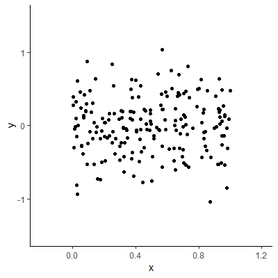
We could also have no clear relationship between $X$ and $Y$. In Figure 1.1.4 below, $Y$ does not appear to be changing in any clear pattern as $X$ changes.
Figure 1.1.4: No Clear Bivariate Relationship
In regression analysis, we will theorize a
The type of relationship between $X$ and $Y$ will help us choose an appropriate model.
Because of this, our first step in a regression analysis for two variables is to examine the