Fill in Blanks
Home
1.1 Bivariate Relationships
1.2 Probabilistic Models
1.3 Estimation of the Line
1.4 Properties of the Least Squares Estimators
1.5 Estimation of the Variance
2.1 The Normal Errors Model
2.2 Inferences for the Slope
2.3 Inferences for the Intercept
2.4 Correlation and Coefficient of Determination
2.5 Estimating the Mean Response
2.6 Predicting the Response
3.1 Residual Diagnostics
3.2 The Linearity Assumption
3.3 Homogeneity of Variance
3.4 Checking for Outliers
3.5 Correlated Error Terms
3.6 Normality of the Residuals
4.1 More Than One Predictor Variable
4.2 Estimating the Multiple Regression Model
4.3 A Primer on Matrices
4.4 The Regression Model in Matrix Terms
4.5 Least Squares and Inferences Using Matrices
4.6 ANOVA and Adjusted Coefficient of Determination
4.7 Estimation and Prediction of the Response
5.1 Multicollinearity and Its Effects
5.2 Adding a Predictor Variable
5.3 Outliers and Influential Cases
5.4 Residual Diagnostics
5.5 Remedial Measures
3.6 Normality of the Residuals
"60% of the time, it works every time." - Brian Fantana (Anchorman)
The difference between model (1.1)
If we do not have normality of the error terms, then the t-tests and t-intervals for $\beta_0$ and $\beta_1$ in Section 2.2 and Section 2.3 would not be valid.
Furthermore, the confidence interval for the mean response (Section 2.5) and the prediction interval for the response (Section 2.6) would not be valid.
If the error terms are not normal, then abootstrapping procedure (see Section 1.4.5) would be necessary to make the inferences discussed in Chapter 2.
We can check the normality of error terms by examining the residuals of the fitted line.
$$
Y_i=\beta_0+\beta_1X_i+\varepsilon_i\qquad\qquad\qquad(1.1)
$$
and model (2.1)
\begin{align*}
Y_i=&\beta_0+\beta_1X_i+\varepsilon_i\\
\varepsilon_i\overset{iid}{\sim}& N\left(0,\sigma^2\right)\qquad\qquad\qquad\qquad(2.1)
\end{align*}
is the assumption of normality of the error terms in (2.1).
If we do not have normality of the error terms, then the t-tests and t-intervals for $\beta_0$ and $\beta_1$ in Section 2.2 and Section 2.3 would not be valid.
Furthermore, the confidence interval for the mean response (Section 2.5) and the prediction interval for the response (Section 2.6) would not be valid.
If the error terms are not normal, then a
We can check the normality of error terms by examining the residuals of the fitted line.
We can graphically check the distribution of the residuals. The two most common ways to do this is with a histogram or with a normal probability plot.
Another (more general) name for a normal probability plot is a normalquantile -quantile (QQ) plot.
For a histogram, we check to see if the shape is approximately close to that of a normal distribution.
For a QQ plot, we check to see if the points approximately follow a straight line. Major departures from a straight line indicatesnonnormality .
It is important to note that we will never see an exact normal distribution is real-world data. Thus, we will always look for approximate normality in the residuals.
The inferences discussed in Chapter 2 are still valid for small departure of normality. However, major departures from normality will lead to incorrectp-values in the hypothesis tests and incorrect coverages in the intervals in Chapter 2.
Another (more general) name for a normal probability plot is a normal
For a histogram, we check to see if the shape is approximately close to that of a normal distribution.
For a QQ plot, we check to see if the points approximately follow a straight line. Major departures from a straight line indicates
It is important to note that we will never see an exact normal distribution is real-world data. Thus, we will always look for approximate normality in the residuals.
The inferences discussed in Chapter 2 are still valid for small departure of normality. However, major departures from normality will lead to incorrect
Below are some examples of histograms and QQ-plots for some simulated datasets.
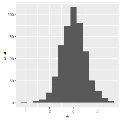
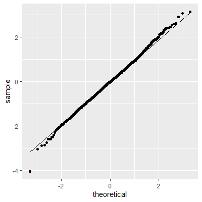
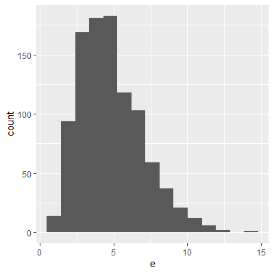
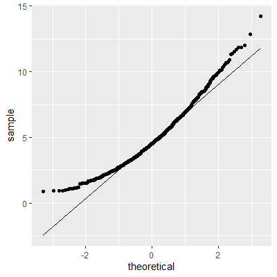
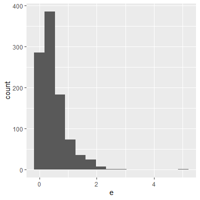
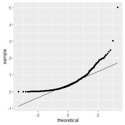
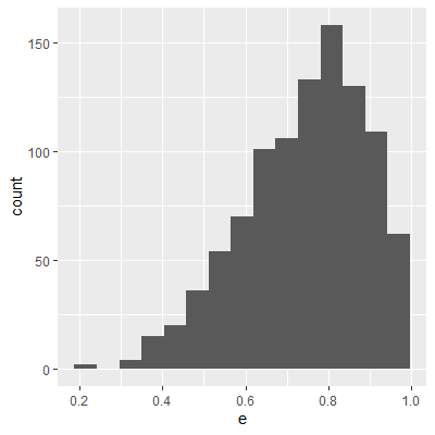
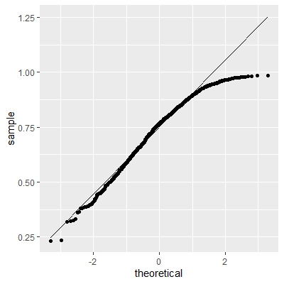
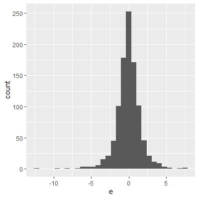
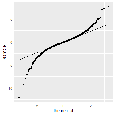
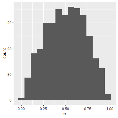
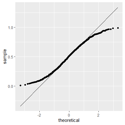
Figure 3.6.1: Normally Distributed
Figure 3.6.2: Right Skewed
Figure 3.6.3: Heavy Right Skewed
Figure 3.6.4: Left Skewed
Figure 3.6.5: Heavy Tails
Figure 3.6.6: No Tails
There are a number of hypothesis test for normality. The most popular test is the Shapiro-Wilk test. This test has been found to have the most power among many of the other tests for normality ( Razali and Wah, 2011)
In the Shapiro-Wilk test, the null hypothesis is that the data are normally distributed and the alternative is that the data are not normally distributed.
This test can be conducted using theshapiro.test function in base R.
Razali, N. M., & Wah, Y. B. (2011). Power comparisons of shapiro-wilk, kolmogorov-smirnov, lilliefors and anderson-darling tests. Journal of statistical modeling and analytics, 2(1), 21-33.
.
In the Shapiro-Wilk test, the null hypothesis is that the data are normally distributed and the alternative is that the data are not normally distributed.
This test can be conducted using the
When there is evidence of nonnormality in the error terms, a transformation on the response variable $Y$ may be useful. This transformation may result in residuals that are closer to being normality distributed.
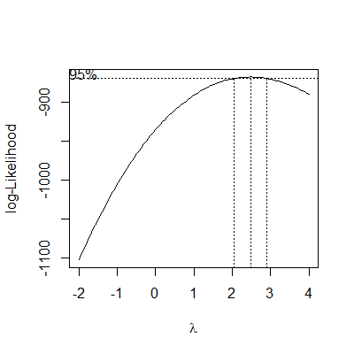
One common way to determine an appropriate transformation is aBox-Cox transformation (Box and Cox, 1964)
In the Box-Cox transformation, a procedure is used to determine a power ($\lambda$) of $Y$ \begin{align*} Y^\prime =& \frac{Y^\lambda - 1}{\lambda} &\text{ if }\lambda\ne 0\\ Y^\prime =& \ln Y & \text{ if }\lambda= 0 \end{align*} that results in a regression fit with residuals as close to normality as possible.
The Box-Cox transformation can be done with theboxcox function in the MASS library.
One common way to determine an appropriate transformation is a
Box, G. E., & Cox, D. R. (1964). An analysis of transformations. Journal of the Royal Statistical Society: Series B (Methodological), 26(2), 211-243.
.
In the Box-Cox transformation, a procedure is used to determine a power ($\lambda$) of $Y$ \begin{align*} Y^\prime =& \frac{Y^\lambda - 1}{\lambda} &\text{ if }\lambda\ne 0\\ Y^\prime =& \ln Y & \text{ if }\lambda= 0 \end{align*} that results in a regression fit with residuals as close to normality as possible.
The Box-Cox transformation can be done with the
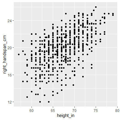
Let's examine the handspan and height data.
We see in the residual plot that there is no clear nonconstant variance pattern (no clear cone pattern). The residuals for taller heights do see to be a little less spread out than the rest. This may be evidence of nonconstant variance. We will conduct a Breusch-Pagan test to see if this is enough evidence to conclude nonconstant variance.
Since the p-value is small, there is sufficient evidence to suggest the variance is nonconstant.
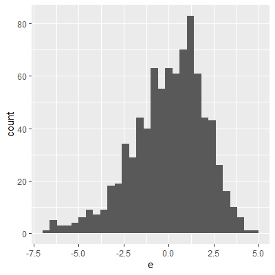
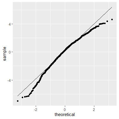
The histogram and QQ plot indicate that the residuals are left-skewed. The p-value for the Shapiro-Wilk test also indicates nonnormality.
After the Box-Cox transformation, the Breusch-Pagan test indicates that there is some evidence of nonconstant variance but not significant enough at the 0.05 level.
With the transformation, the residuals are still not perfectly normal, however, the skewness is not as heavy as the untransformed data.
The Shapiro-Wilk test still indicates that the residuals are not normally distributed. We stated early that small departures from normality are okay. From the QQ plot, the residuals are not as skewed as before the transformation. Therefore, this transformation helped and we can perform the inferences assuming normality.
We also note that the Shapiro-Wilk test is just like any other hypothesis test in that the more data you have, the more likely you will reject the null hypothesis. The null hypothesis is that the residuals are normally distributed. We stated before that no "real-world" data are perfectly normally distributed. Thus, the null hypothesis is not correct. We just want to know if there is enough evidence against normality. The more data you have, the more likely that you have enough evidence to reject the null. This is why we should not just depend on the Shapiro-Wilk test but examine a QQ plot as well.
library(tidyverse)
library(lmtest)
library(MASS)

dat = read_csv("http://www.jpstats.org/Regression/data/Survey_Measurements.csv",)

ggplot(dat, aes(x=height_in, y=right_handspan_cm))+
  geom_point()


#fit the model
fit = lm(right_handspan_cm~height_in, data=dat)
fit %>% summary

Call:
lm(formula = right_handspan_cm ~ height_in, data = dat)

Residuals:
    Min      1Q  Median      3Q     Max
-6.9918 -1.2418  0.2427  1.3989  4.6255

Coefficients:
            Estimate Std. Error t value Pr(>|t|)
(Intercept)  -3.1322     1.1557   -2.71  0.00686 **
height_in     0.3457     0.0172   20.10  < 2e-16 ***
---
Signif. codes:  0 ‘***’ 0.001 ‘**’ 0.01 ‘*’ 0.05 ‘.’ 0.1 ‘ ’ 1

Residual standard error: 2.008 on 832 degrees of freedom
Multiple R-squared:  0.3269,	Adjusted R-squared:  0.3261
F-statistic:   404 on 1 and 832 DF,  p-value: < 2.2e-16


#get the residuals and add to dataframe
dat$e = resid(fit)

#residual plot
ggplot(dat, aes(x=height_in, y=e))+
  geom_point()+
  geom_smooth(method="lm", formula=y~x, se=F)
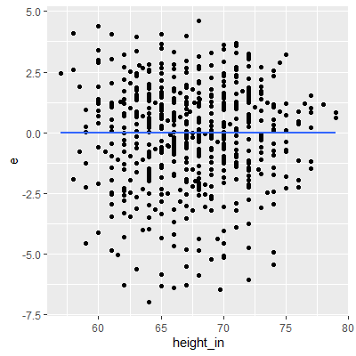
We see in the residual plot that there is no clear nonconstant variance pattern (no clear cone pattern). The residuals for taller heights do see to be a little less spread out than the rest. This may be evidence of nonconstant variance. We will conduct a Breusch-Pagan test to see if this is enough evidence to conclude nonconstant variance.
#test for nonconstant variance
bptest(fit)

	studentized Breusch-Pagan test

data:  fit
BP = 4.5167, df = 1, p-value = 0.03357
Since the p-value is small, there is sufficient evidence to suggest the variance is nonconstant.
#check for normality
ggplot(dat, aes(x=e))+
  geom_histogram()


ggplot(dat, aes(sample=e))+
  geom_qq()+
  geom_qq_line()


#test for normality
shapiro.test(dat$e)

	Shapiro-Wilk normality test

data:  dat$e
W = 0.97649, p-value = 2.459e-10
The histogram and QQ plot indicate that the residuals are left-skewed. The p-value for the Shapiro-Wilk test also indicates nonnormality.
#attempt a box cox transformation
bc = boxcox(fit,lambda = seq(-2,4,by=0.1))
lam = with(bc, x[which.max(y)])
#do the transformation and add to dataframe
dat$Y.prime = (dat$right_handspan_cm^lam - 1) / lam
#fit with transformed y
fit2 = lm(Y.prime~height_in, data=dat)
fit2 %>% summary
Call:
lm(formula = Y.prime ~ height_in, data = dat)
Residuals:
Min 1Q Median 3Q Max
-481.99 -112.55 8.13 115.00 458.65
Coefficients:
Estimate Std. Error t value Pr(>|t|)
(Intercept) -1292.984 95.341 -13.56 <2e-16 ***
height_in 29.878 1.419 21.06 <2e-16 ***
---
Signif. codes: 0 ‘***’ 0.001 ‘**’ 0.01 ‘*’ 0.05 ‘.’ 0.1 ‘ ’ 1
Residual standard error: 165.7 on 832 degrees of freedom
Multiple R-squared: 0.3477, Adjusted R-squared: 0.3469
F-statistic: 443.5 on 1 and 832 DF, p-value: < 2.2e-16
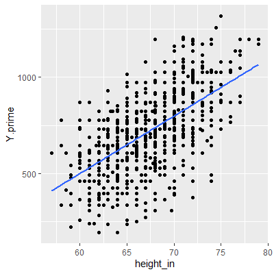
#plot with regression line
ggplot(dat, aes(x=height_in, y=Y.prime))+
geom_point()+
geom_smooth(method="lm", formula=y~x, se=F)
#get the residuals and add to dataframe
dat$e2 = resid(fit2)
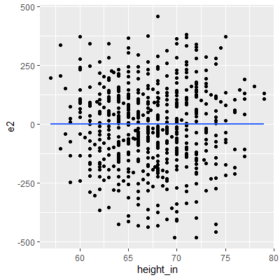
ggplot(dat, aes(x=height_in, y=e2))+
geom_point()+
geom_smooth(method="lm", formula=y~x, se=F)
#check for nonconstant variance
bptest(fit2)
studentized Breusch-Pagan test
data: fit2
BP = 3.4908, df = 1, p-value = 0.06171
After the Box-Cox transformation, the Breusch-Pagan test indicates that there is some evidence of nonconstant variance but not significant enough at the 0.05 level.
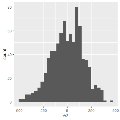
#check for normality
ggplot(dat, aes(x=e2))+
  geom_histogram()


ggplot(dat, aes(sample=e2))+
  geom_qq()+
  geom_qq_line()
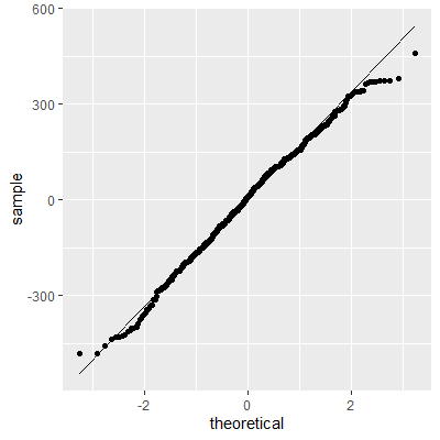
With the transformation, the residuals are still not perfectly normal, however, the skewness is not as heavy as the untransformed data.
#test for normality
shapiro.test(dat$e2)

	Shapiro-Wilk normality test

data:  dat$e2
W = 0.99486, p-value = 0.006499
The Shapiro-Wilk test still indicates that the residuals are not normally distributed. We stated early that small departures from normality are okay. From the QQ plot, the residuals are not as skewed as before the transformation. Therefore, this transformation helped and we can perform the inferences assuming normality.
We also note that the Shapiro-Wilk test is just like any other hypothesis test in that the more data you have, the more likely you will reject the null hypothesis. The null hypothesis is that the residuals are normally distributed. We stated before that no "real-world" data are perfectly normally distributed. Thus, the null hypothesis is not correct. We just want to know if there is enough evidence against normality. The more data you have, the more likely that you have enough evidence to reject the null. This is why we should not just depend on the Shapiro-Wilk test but examine a QQ plot as well.