2.4 Correlation and Coefficient of Determination

Now that we can fit the model to the data, we want to assess how "good" of a fit we have.

We will present two measures that will quantify how well the model fits the data.

For the data $(X_i,Y_i)$, $i=1,\ldots,n$, we want a measure of how well a linear model explains a linear relationship between $X$ and $Y$.

We start by defining $$ SS_{XX} = \sum\left(X_i-\bar{X}\right)^2\qquad\qquad\qquad(2.11) $$ and $$ SS_{YY} = \sum\left(Y_i-\bar{Y}\right)^2\qquad\qquad\qquad(2.12) $$ $SS_{XX}$ and $SS_{YY}$ are measures of variability of $X$ and $Y$, respectively. That is, they indicate how $X$ and $Y$ vary about their mean, individually.

Now, we define $$ SS_{XY}=\sum\left(X_i-\bar{X}\right)\left(Y_i-\bar{Y}\right)\qquad\qquad\qquad(2.13) $$ $SS_{XY}$ is a measure of how $X$ and $Y$ varies together.

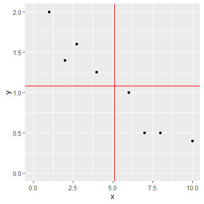
For example, consider the data from Figure 1.3.1 . Let's find $SS_{XX}$, $SS_{YY}$, and $SS_{XY}$ in R.

library(tidyverse)

x = c(1,2 ,2.75, 4, 6, 7, 8, 10)
y = c(2, 1.4, 1.6, 1.25, 1, 0.5, 0.5, 0.4)

dat =  tibble(x,y)

ybar =  mean(y)
xbar =  mean(x)

ggplot(dat, aes(x=x,y=y))+
  geom_point()+
  xlim(0,10)+
  ylim(0,2)+
  geom_hline(yintercept = ybar,col="red")+
  geom_vline(xintercept = xbar, col="red")

dev_x = x-xbar
dev_y = y-ybar 

dev_xy = dev_x*dev_y 

dat1 = tibble(x,y,dev_x^2,dev_y^2,dev_xy)
dat1

      x     y `dev_x^2` `dev_y^2`  dev_xy
1  1     2       16.8     0.844   -3.76  
2  2     1.4      9.57    0.102   -0.986 
3  2.75  1.6      5.49    0.269   -1.22  
4  4     1.25     1.20    0.0285  -0.185 
5  6     1        0.821   0.00660 -0.0736
6  7     0.5      3.63    0.338   -1.11  
7  8     0.5      8.45    0.338   -1.69  
8 10     0.4     24.1     0.464   -3.34  
                                

In the output of dat1, dev_x^2 represents $(X_i-\bar{X})^2$ and dev_y^2 represents $(Y_i-\bar{Y})^2$ for each observation.

dev_xy represents $(X_i-\bar{X})(Y_i-\bar{Y})$ for each observation. Note that each value is negative. This is because as $X$ is below $\bar{X}$, $Y$ is above $\bar{Y}$. Likewise, as $X$ is above $\bar{X}$, $Y$ is below $\bar{Y}$. In the ggplot above, the two red lines represent $\bar{X}$ (the vertical red line) and $\bar{Y}$ (the horizontal red line). You can see how the observations are below or above these lines.

We can find the values of $SS_{XX}$, $SS_{YY}$, and $SS_{XY}$ by

#SS_XX
dev_x^2 %>% sum()
[1] 69.99219

#SS_YY
dev_y^2 %>% sum()
[1] 2.389687

#SS_XY
dev_xy %>% sum()
[1] -12.36094

                            

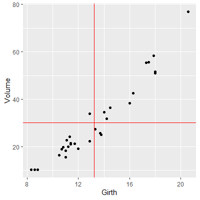
For another example, consider the trees dataset from Example 2.2.1. Again, we plot the data with red lines representing $\bar{X}$ and $\bar{Y}$.

library(datasets)
library(tidyverse)

xbar = mean(trees$Girth)
ybar = mean(trees$Volume)

ggplot(data=trees, aes(x=Girth, y=Volume))+
  geom_point()+
  geom_hline(yintercept = ybar,col="red")+
  geom_vline(xintercept = xbar, col="red")




x = trees$Girth
y = trees$Volume

dev_x = x-xbar
dev_y = y-ybar 

dev_xy = dev_x*dev_y 


dat1 = tibble(x,y,dev_x^2,dev_y^2,dev_xy)
dat1 %>% print(n=31)
       x     y `dev_x^2` `dev_y^2`  dev_xy
 1   8.3  10.3  24.5        395.    98.3  
 2   8.6  10.3  21.6        395.    92.4  
 3   8.8  10.2  19.8        399.    88.8  
 4  10.5  16.4   7.55       190.    37.8  
 5  10.7  18.8   6.49       129.    29.0  
 6  10.8  19.7   5.99       110.    25.6  
 7  11    15.6   5.06       212.    32.8  
 8  11    18.2   5.06       143.    26.9  
 9  11.1  22.6   4.62        57.3   16.3  
10  11.2  19.9   4.20       105.    21.0  
11  11.3  24.2   3.80        35.7   11.6  
12  11.4  21     3.42        84.1   17.0  
13  11.4  21.4   3.42        76.9   16.2  
14  11.7  21.3   2.40        78.7   13.7  
15  12    19.1   1.56       123.    13.8  
16  12.9  22.2   0.121       63.5    2.78 
17  12.9  33.8   0.121       13.2   -1.26 
18  13.3  27.4   0.00266      7.68  -0.143
19  13.7  25.7   0.204       20.0   -2.02 
20  13.8  24.9   0.304       27.8   -2.91 
21  14    34.5   0.565       18.7    3.25 
22  14.2  31.7   0.906        2.34   1.46 
23  14.5  36.3   1.57        37.6    7.67 
24  16    38.3   7.57        66.1   22.4  
25  16.3  42.6   9.31       154.    37.9  
26  17.3  55.4  16.4        637.   102.   
27  17.5  55.7  18.1        652.   109.   
28  17.9  58.3  21.6        791.   131.   
29  18    51.5  22.6        455.   101.   
30  18    51    22.6        434.    99.0  
31  20.6  77    54.0       2193.   344. 

#SS_XX
dev_x^2 %>% sum()
[1] 295.4374


#SS_YY
dev_y^2 %>% sum()
[1] 8106.084


#SS_XY
dev_xy %>% sum()
[1] 1496.644

In this example, most of the observations have $(X-\bar{X})(Y-\bar{Y})$ that are positive. This is because these observations have values of $X$ that are below $\bar{X}$ and values of $Y$ that are below $\bar{Y}$, or values of $X$ that are above $\bar{X}$ and values of $Y$ that are above $\bar{Y}$.

There are four observations that have a negative value of $(X-\bar{X})(Y-\bar{Y})$. Although they are negative, the value of $SS_{XY}$ is positive due to all the observations with positive values of $(X-\bar{X})(Y-\bar{Y})$. Therefore, we say if $SS_{XY}$ is positive, then $Y$ tends to increase as $X$ increases. Likewise, if $SS_{XY}$ is negative, then $Y$ tends to decrease as $X$ increases.

If $SS_{XY}$ is zero (or close to zero), then we say $Y$ does not tend to change as $X$ increases.

We first note that $SS_{XY}$ cannot be greater in absolute value than the quantity $$ \sqrt{SS_{XX}SS_{YY}} $$ We will not prove this here, but it is a direct application of the Cauchy-Schwarz inequality.

We define the linear correlation coefficient as $$ r=\frac{SS_{XY}}{\sqrt{SS_{XX}SS_{YY}}}\qquad\qquad\qquad(2.13) $$.

$r$ is also called the Pearson correlation coefficient.

We note that $$ -1\le r \le 1 $$

If $r=0$, then there is no linear relationship between $X$ and $Y$.

If $r$ is positive, then the slope of the linear relationship is positive. If $r$ is negative, then the slope of the linear relationship is negative.

The closer $r$ is to one in absolute value, the stronger the linear relationship is between $X$ and $Y$.

Note how the value of $r$ relates to how spread out the points are from the line as well as to the slope of the line.

The correlation $r$ is for the observed data which is usually from a sample. Thus, $r$ is the sample correlation coefficient.

We could make a hypothesis about the correlation of the population based on the sample. We will denote the population correlation with $\rho$. The hypothesis we will want to test is $$ H_0:\rho = 0\\ H_1:\rho \ne 0 $$

Recall from Section 2.2.4 that (2.6) can be used to test a hypothesis for the slope.

If we test \begin{align*} H_{0}: & \beta_{1}=0\\ H_{a}: & \beta_{1}\ne0 \end{align*} then this is equivalent to testing \begin{align*} H_{0}: & \rho=0\\ H_{a}: & \rho\ne0 \end{align*} since both hypotheses test to see of there is no linear relationship between $X$ and $Y$.

Now note, using (1.4) , that $b_{1}$ can be rewritten as \begin{align*} b_{1} & =\frac{\sum\left(X_{i}-\bar{X}\right)\left(Y_{i}-\bar{Y}\right)}{\sum\left(X_{i}-\bar{X}\right)^{2}}\\ & =\frac{SS_{XY}}{SS_{XX}}\\ & =\frac{rSS_{XY}}{rSS_{XX}}\\ & =\frac{rSS_{XY}}{\frac{SS_{XY}}{\sqrt{SS_{xx}SS_{YY}}}SS_{XX}}\\ & =\frac{r\sqrt{SS_{XX}SS_{YY}}}{SS_{XX}}\\ & =r\frac{\sqrt{\frac{SS_{XX}}{n-1}\frac{SS_{YY}}{n-1}}}{\frac{SS_{XX}}{n-1}}\\ & =r\frac{s_{X}s_{Y}}{s_{X}^{2}}\\ & =r\frac{s_{y}}{s_{X}}\qquad\qquad\qquad(2.14) \end{align*} where $s_{Y}$ and $s_{X}$ are the sample standard deviation of $Y$ and $X$, respectively.

Also, $SSE$ from (1.16) can be rewritten as \begin{align*} SSE & =\sum\left(Y_{i}-\hat{Y}_{i}\right)^{2}\\ & =\sum\left(Y_{i}-\underbrace{b_{0}}_{(1.4)}-b_{1}X_{i}\right)^{2}\\ & =\sum\left(Y_{i}-\overline{Y}+b_{1}\overline{X}-b_{1}X_{i}\right)^{2}\\ & =\sum\left(\left(Y_{i}-\overline{Y}\right)-b_{1}\left(X_{i}-\overline{X}\right)\right)^{2}\\ & =\sum\left(\left(Y_{i}-\overline{Y}\right)^{2}-2b_{1}\left(X_{i}-\overline{X}\right)\left(Y_{i}-\overline{Y}\right)+b_{1}^{2}\left(X_{i}-\overline{X}\right)^{2}\right)\\ & =SS_{YY}-2\underbrace{b_{1}}_{(1.4)}SS_{XY}+b_{1}^{2}SS_{XX}\\ & =SS_{YY}-2\left(\frac{SS_{XY}}{SS_{XX}}\right)SS_{XY}+\left(\frac{SS_{XY}}{SS_{XX}}\right)^{2}SS_{XX}\\ & =SS_{YY}-\left(\frac{SS_{XY}}{SS_{XX}}\right)SS_{XY}\\ & =SS_{YY}-\underbrace{b_{1}}_{(2.14)}SS_{XY}\\ & =SS_{YY}-r\left(\frac{\sqrt{SS_{YY}}}{\sqrt{SS_{XX}}}\right)SS_{XY}\\ & =SS_{YY}\left(1-r\frac{SS_{XY}}{\sqrt{SS_{XX}}\sqrt{SS_{YY}}}\right)\\ & =SS_{YY}\left(1-r^{2}\right)\qquad\qquad\qquad\qquad(2.15) \end{align*} Now, using (2.14) and (2.15), we write the test statistic as \begin{align*} t & =\frac{b_{1}}{\sqrt{\frac{s^{2}}{\sum\left(X_{i}-\bar{X}\right)^{2}}}}\\ & =\frac{r\frac{s_{y}}{s_{X}}}{\sqrt{\frac{SSE}{\left(n-2\right)SS_{XX}}}}\\ & =\frac{r\frac{s_{y}}{s_{X}}}{\sqrt{\frac{SS_{YY}\left(1-r^{2}\right)}{\left(n-2\right)SS_{XX}}}}\\ & =\frac{r\frac{s_{y}}{s_{X}}}{\sqrt{\frac{\left(1-r^{2}\right)s_{Y}^{2}}{\left(n-2\right)s_{X}^{2}}}}\\ & =\frac{r\frac{s_{y}}{s_{X}}\sqrt{\left(n-2\right)}}{\frac{s_{y}}{s_{X}}\sqrt{1-r^{2}}}\\ & =\frac{r\sqrt{\left(n-2\right)}}{\sqrt{1-r^{2}}}\qquad\qquad\qquad(2.16) \end{align*}

If $H_0$ is true, then $t$ will have a Student's $t$-distribution with $n-2$ degrees of freedom.

The second measure of how well the model fits the data involves measuring the amount of variability in $Y$ that is explained by the model using $X$. We start by examining the variability of the variable we want to learn about. We want to learn about the response variable $Y$. One way to measure the variability of $Y$ is with $$ SS_{YY} = \sum\left(Y_i-\bar{Y}\right)^2\qquad\qquad\qquad(2.12) $$ Note that $SS_{YY}$ does not include the model or $X$. It is just a measure of how $Y$ deviates from its mean $\bar{Y}$.

We also have the variability of the points about the line. We can measure this with the sum of squares error $$ SSE = \sum \left(Y_i - \hat{Y}_i\right)^2\qquad\qquad\qquad(1.16) $$ Note that SSE does include $X$. This is because the fitted line $\hat{Y}$ is a function of $X$.

Let's look again at the Handspan and Height data from Section 1.1. If using $X$ in the model does not help in explaining $Y$, then the regression line will be horizontal. That is, the slope will be zero. In that case, $SS_{YY}$ and SSE will be the same.

If using $X$ in the model helps substantially in explaining $Y$, then the points should be somewhat close to the regression line. Therefore, SSE will be much smaller than $SS_{YY}$.

We want to explain as much of the variation of $Y$ as possible. So we want to know just how much of that variation is explained by using linear regression model with $X$. We can quantify this variation explained by taking the difference $$ SSR = SS_{YY}-SSE\qquad\qquad\qquad(2.17) $$ SSR is called the sum of squares regression.

We calculate the proportion of the variation of $Y$ explained by the regression model using $X$ by calculating $$ R^2 = \frac{SSR}{SS_{YY}}\qquad\qquad\qquad(2.18) $$ $R^2$ is called the coefficient of determination.