5.3 Outliers and Influential Observations

"You keep using that word. I do not think it means what you think it means."
- Inigo Montoya (The Princess Bride )

5.3.1 Outliers with Respect to $Y$

In Section 3.4 we discussed outliers in the simple regression case. Recall from Figure 3.4.1 that a point can be outlying with respect to $Y$ or with respect to $X$ but have little effect on the fitted line.

If an observation is outlying with respect to $Y$ but has an $X$ value close to $\bar{X}$, then it will have little effect on $\hat{Y}$. If it is far from $\bar{X}$, it will have a large effect.

If an observation is an outlier with respect to $X$ but still follows the linear relationship between $X$ and $Y$, then it will also have little effect on $\hat{Y}$.

In multiple regression, we will still need to view the outliers with respect to $Y$ and with respect to the predictor variables $X_1\ldots,X_{p-1}$. We will identify these outlying observations by how they affect the fitted model $\hat{Y}$.

Studentized Residuals

Recall from Section 3.4.2 that semistudentized residuals \begin{align*} e_{i}^{*} & =\frac{e_{i}}{\sqrt{MSE}}\qquad\qquad\qquad(3.3) \end{align*} can be used to determine if an observation is an outlier.

We called them semistudentized because $\sqrt{MSE}$ is not an estimate of the true standard error of $e_i$. Therefore dividing by $\sqrt{MSE}$ does not give a true student t-score.

With the hat matrix \begin{align*} {\bf H} & ={\bf X}\left({\bf X}^{\prime}{\bf X}\right)^{-1}{\bf X}^{\prime}\qquad(4.24) \end{align*} we can now present the true variance of $e_i$: \begin{align*} Var\left[e_{i}\right] & =\sigma^{2}\left(1-h_{ii}\right)\qquad(5.3) \end{align*} where $h_{ii}$ is the $i$th diagonal element of $\bf{H}$.

We can estimate $Var\left[e_{i}\right]$ with \begin{align*} s^2\left[e_{i}\right] & =MSE\left(1-h_{ii}\right)\qquad(5.4) \end{align*}

Dividing $e_i$ by $s\left[e_{i}\right]$ gives us a true t-score. Thus the studentized residual is \begin{align*} r_{i} & =\frac{e_{i}}{\sqrt{MSE\left(1-h_{ii}\right)}}\qquad(5.5) \end{align*} A rule of thumb is any $r_i$ greater than 3 in absolute value should be considered an outlier with respect to $Y$.

Deleted Residuals

As we stated above, it is possible for an observation to be outlying with respect to $Y$ but not have an effect on the fitted value.

Also, if $Y$ does effect the fit greatly, then the fitted value $\hat{Y}$ will be "pulled" towards $Y$ and thus make $r_i$ not so large.

One way to see how an (potentially outlying) observation $Y_i$ influences the fit is by first fitting the model without $Y_i$ and then try to predict $Y_i$ based on that fitted model.

The difference from the observed $Y_i$ and the predicted value based on the model fitted with the remaining $n-1$ observations $\hat{Y}_{i(i)}$ is called the deleted residual: \begin{align*} d_{i} & =Y_{i}-\hat{Y}_{i\left(i\right)}\qquad(5.6) \end{align*} At first glance, it would appear that obtaining $d_i$ for all observations would be computationally expensive since it would require a different fitted model for each $i=1,\ldots,n$. However, it can be shown that the deleted residuals can be expressed as \begin{align*} d_{i} & =\frac{e_{i}}{1-h_{ii}}\qquad(5.7) \end{align*} which would not require a new fit for each $i$.

Studentized Deleted Residuals

The estimated variance of the deleted residual $d_{i}$ is \begin{align*} s^{2}\left[d_{i}\right] & =\frac{MSE_{(i)}}{1-h_{ii}}\qquad(5.8) \end{align*} where $MSE_{(i)}$ is the $MSE$ of the fit with $Y_{i}$ removed.

We can obtain a studentized deleted residual with \begin{align*} t_{i} & =\frac{d_{i}}{s\left[d_{i}\right]}\\ & =\frac{e_{i}}{\sqrt{MSE_{(i)}\left(1-h_{ii}\right)}}\qquad(5.9) \end{align*} Again, we do not need to calculate a new regression fit for each $i$ due to the relationship \begin{align*} MSE_{(i)} & =\left(\frac{n-p}{n-p-1}\right)MSE-\frac{e_{i}^{2}}{\left(n-p-1\right)\left(1-h_{ii}\right)}\qquad(5.10) \end{align*} Since $t_{i}$ follows a Student's $t$ distribution with $n-p-1$ degrees of freedom, then any $t_{i}$ greater than $t_{\alpha/2n}$ will be considered a potential outlier.

Note that the $\alpha/2n$ is called a Bonferroni adjustment in that it divides the significance level $\alpha$ by $2n$. This is done to control for an overall significance level of $\alpha$ when examining the $n$ studentized deleted residuals.

5.3.2 Outliers with Respect to $\bf{X}$

We can identify outliers with respect to the predictor variables with the help of the hat matrix ${\bf H}$.

We have already seen that it plays an important role in the studentized deleted residuals.

We will now use the diagonal elements of ${\bf H}$, $h_{ii}$, as a measure of how far the $X$ values of an observation are from the center $X$ value of all the observations.

Leverage Values

We first note some properties or $h_{ii}$: \begin{align*} & 0\le h_{ii}\le1 & \qquad(5.11)\\ & \sum h_{ii}=p & \qquad(5.12) \end{align*} The larger the value of $h_{ii}$, the further the $i$th observation is from the center of all the $X$'s. Thus, we call $h_{ii}$ the leverage. If an observation has a large leverage value, then it has a substantial ``leverage'' in determining $\hat{Y}_{i}$.

Leverage values greater than $2p/n$ are considered large when $n$ is reasonably large.

Using Leverage to Identify Hidden Extrapolation

In simple regression, we stated that we did not want to extrapolate outside the range of the $X$ variable.

In multiple regression, we still do not want to extrapolate but now we cannot just think in terms of the range of each individual predictor variable. We must now think in terms of extrapolating for values combinations of the $X$ variables that we may not have seen information for in our data.

For example in the bodyfat data, tri had a range of about 14 to 32. The variable thigh had a range of values from about 42 to about 58.5. However, we did not have any observations with a tri of, say, 16 and a thigh of, say, 55. Those with small tri values also tended to have small thigh values. So this would be hidden extrapolation.

We can use the hat matrix to identify hidden extrapolation. This is done by using the vector of $X$ values you want to predict at, ${\bf X}_{new}$, and then including it in the hat matrix as \begin{align*} h_{new,new} & ={\bf X}_{new}^{\prime}\left({\bf X}^{\prime}{\bf X}\right)^{-1}{\bf X}_{new}\qquad(5.13) \end{align*} If the value of $h_{new,new}$ is much larger than the leverage values in the data set, then it indicates extrapolation.

5.3.3 Influential Cases

Once we have identified observations that are outlying with respect to $Y$ or with respect to predictor variables, or both, we now want to know just how much it affects the fitted regression model.

If an observation causes major changes in the fitted model when excluded, then we say the observation is influential.

Not all outliers are influential. We will determine which are influential by seeing what happens to the fitted values when that observation is deleted as we did with the deleted residuals above.

Influence on a Single Fitted Value

We can see how much influence an observation has on a single fitted value $\hat{Y}_{i}$ by examining \begin{align*} DFFITS_{i} & =\frac{\hat{Y}_{i}-\hat{Y}_{i\left(i\right)}}{\sqrt{MSE_{(i)}h_{ii}}}\qquad(5.14) \end{align*} As before, a new regression fit is not needed to obtain $DFFITS_{i}$. It can be shown that (5.14) can be expressed as \begin{align*} DFFITS_{i} & =t_{i}\left(\frac{h_{ii}}{1-h_{ii}}\right)^{1/2}\qquad(5.15) \end{align*} which does not require a new regression fit excluding the $i$th observation.

A general guideline is that a value of DFFITS greater than 1 for small to medium datasets and greater than $2\sqrt{p/n}$ for large datasets indicates an influential observation.

Influence on All Fitted Values

We can consider the influence of the $i$th observation on all the fitted values $\hat{Y}_{i}$ with a measure known as Cook's distance.

It is defined as \begin{align*} D_{i} & =\frac{\sum_{j=1}^{n}\left(\hat{Y}_{j}-\hat{Y}_{j\left(i\right)}\right)^{2}}{pMSE}\\ & =\frac{e_{i}^{2}}{pMSE}\left(\frac{h_{ii}}{\left(1-h_{ii}\right)^{2}}\right)\qquad(5.16) \end{align*} Note the last expression in (5.16) does not require a new fitted regression model for each $i$.

From (5.16), we see that $D_{i}$ depends on $e_{i}$ and $h_{ii}$. If either one is large, then $D_{i}$ will be large.

So an influential observation can have a (1) large residual $e_{i}$ and a moderate leverage $h_{ii}$, (2) a large leverage $h_{ii}$ and a moderate residual $e_{i}$, (3) or both a large residual and large leverage.

Influence on the Coefficients

We can also see the influence of an observation on the individual coefficients $b_{k}$, $k=0,1,\ldots,p-1$. Again, we do this by seeing how much $b_{k}$ changes when that observation is removed.

A measure of this change is \begin{align*} DFBETAS_{k\left(i\right)} & =\frac{b_{k}-b_{k\left(i\right)}}{\sqrt{MSE_{(i)}c_{kk}}} \end{align*} where $c_{kk}$ is the $k$th diagonal element of $\left({\bf X}^{\prime}{\bf X}\right)^{-1}$.

The sign of $DFBETAS$ indicates whether $b_{k}$ increases or decreases when the $i$th observation is removed from the data. A large magnitude of $DFBETAS$ indicates the $i$th observation is influential on the $k$th coefficient.

A rule of thumb is a $DFBETAS$ value greater than 1 in absolute value for small to medium datasets and greater than $2/\sqrt{n}$ for large datasets indicates an influential observation.

Example 5.3.1

Let's examine the bodyfat data and determine if there is any observations that we should be concerned about.

We have already seen that there is an issue of multicollinearity in this data. Regardless, let's just fit the model to all three variables for this example.

To obtain plots for all the measures discussed in this section, we will use the olsrr library.

library(tidyverse)
library(car)
library(olsrr)

dat = read.table("http://www.jpstats.org/Regression/data/BodyFat.txt", header=T)

#fit the full model
fit = lm(bfat~., data=dat)

#first examine outliers with respect to Y
#can obtain studentized deleted residuals with
rstudent(fit) %>% tibble()

 1 -1.53  
 2  1.14  
 3 -1.25  
 4 -1.33  
 5  0.564 
 6 -0.228 
 7  0.610 
 8  1.42  
 9  0.755 
10 -0.565 
11  0.340 
12  0.940 
13 -1.57  
14  2.02  
15  0.482 
16  0.0716
17 -0.156 
18 -0.624 
19 -1.71  
20  0.248


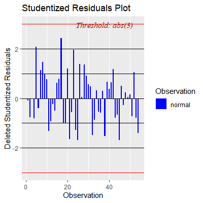
#plot the studentized deleted residuals
ols_plot_resid_stud(fit)



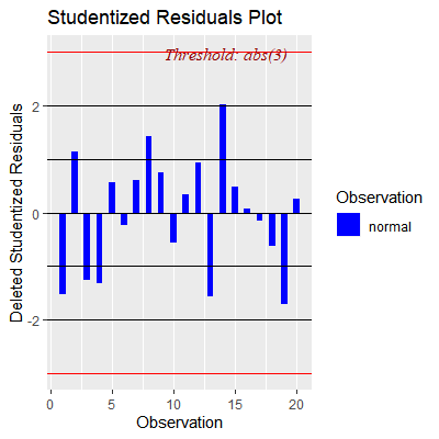
#no outliers w.r.t Y

#to get the leverage values
hatvalues(fit) %>% tibble()

 1 0.341 
 2 0.157 
 3 0.440 
 4 0.112 
 5 0.361 
 6 0.132 
 7 0.194 
 8 0.164 
 9 0.193 
10 0.241 
11 0.139 
12 0.109 
13 0.214 
14 0.188 
15 0.348 
16 0.114 
17 0.125 
18 0.228 
19 0.132 
20 0.0660


#plot the deleted studentized residuals vs hat values 
ols_plot_resid_lev(fit)



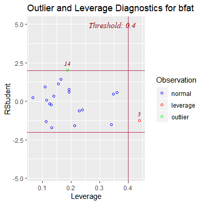
#note that the thresholds given for the residuals are not the Bonferroni limits
#discussed above
#the threshold for the levearge is the rule of thumb above which is 2p/n

#Here, we see obs 3 has high leverage but not an outlier wrt Y
#Obs 14 could possibly be an outlier wrt Y but does not have 
#high leverage


#we now want to see of obs 3 and 17 are influential

#first to see if influential to their own fitted values

#to get dffits
dffits(fit) %>% tibble()

 1 -1.10  
 2  0.493 
 3 -1.11  
 4 -0.472 
 5  0.424 
 6 -0.0888
 7  0.300 
 8  0.631 
 9  0.369 
10 -0.318 
11  0.137 
12  0.329 
13 -0.819 
14  0.970 
15  0.352 
16  0.0257
17 -0.0591
18 -0.339 
19 -0.667 
20  0.0659


#to plot dffits
#the threshold is 2*sqrt(p/n)
ols_plot_dffits(fit)




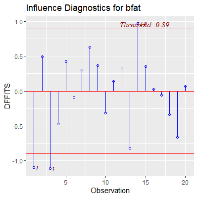
#obs 3 is influential to its own fitted value but obs 17 is not

#to get Cook's distance (influence on all fitted values)
cooks.distance(fit) %>% tibble()

 1 0.279   
 2 0.0596  
 3 0.299   
 4 0.0532  
 5 0.0469  
 6 0.00210 
 7 0.0234  
 8 0.0936  
 9 0.0350  
10 0.0264  
11 0.00495 
12 0.0273  
13 0.154   
14 0.198   
15 0.0325  
16 0.000176
17 0.000929
18 0.0299  
19 0.0992  
20 0.00115 


#plot Cook's distance
#the threshold is based on the F distribution with p and n-p degrees of freedom
ols_plot_cooksd_chart(fit)



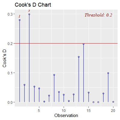
#so obs 3 is influential to all fitted values and obs 17 is not. 

#we now check the effect on the estimated coefficients

#obtain the dfbetas
dfbeta(fit) %>% tibble()

   .[,"(Intercept)"] [,"tri"] [,"thigh"] [,"midarm"]
 1           -72.9    -2.12      1.88        1.08   
 2            39.4     1.18     -1.02       -0.615  
 3            37.4     1.02     -0.868      -0.688  
 4             4.48    0.0758   -0.0827     -0.0847 
 5           -21.6    -0.683     0.552       0.387  
 6            -0.835  -0.0218    0.0148      0.0217 
 7           -14.9    -0.420     0.384       0.218  
 8            40.9     1.27     -1.09       -0.628  
 9            22.8     0.652    -0.561      -0.380  
10            25.0     0.762    -0.660      -0.382  
11            -5.36   -0.143     0.132       0.0829 
12            -0.566   0.0225    0.00686    -0.00836
13            32.5     1.10     -0.910      -0.508  
14           -36.2    -1.19      0.948       0.655  
15            -7.52   -0.294     0.229       0.120  
16             1.10    0.0363   -0.0299     -0.0173 
17             2.71    0.0803   -0.0723     -0.0386 
18           -10.7    -0.342     0.266       0.205  
19           -45.5    -1.33      1.16        0.707  
20             3.37    0.100    -0.0861     -0.0531 


#plot dfbetas
#the thresholds is 2*sqrt(n)
ols_plot_dfbetas(fit)



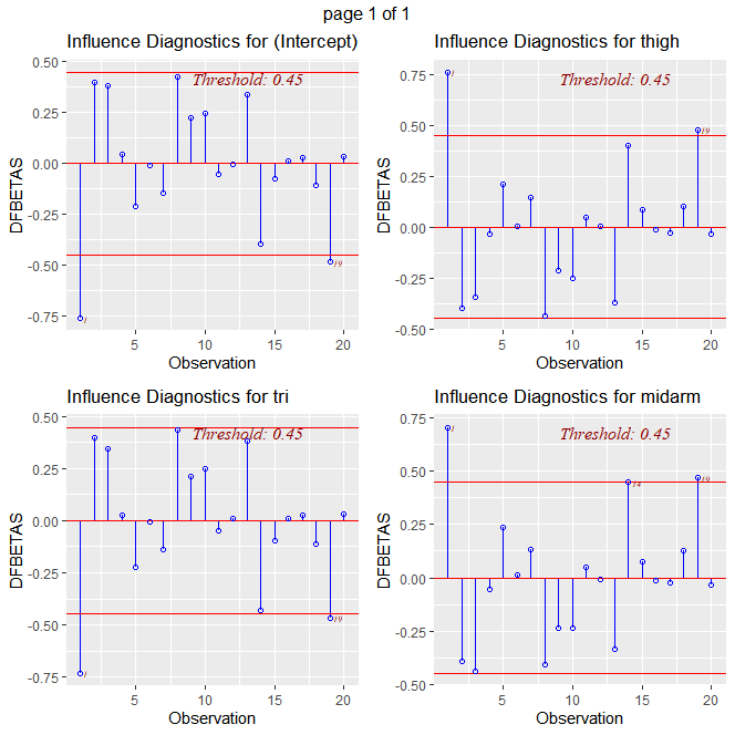
#it appear obs 3 had the largest influence on midarm, however,
#it is not beyond the rule of thumb threshold

#It appears obs 3 is an outlier wrt X and influential on the fitted values
#We should examine obs 3 and determine if a remedial measure is needed

# Suppose we want to predict bodyfat for a woman in this population with
# tri = 19.5, thigh = 44, and midarm = 29. 
#first setup the dataframe
xnew = data.frame(tri=19.5, thigh=44, midarm=29) %>% as.matrix() %>% t()
xnew = rbind(1,xnew)

dat.mat = dat %>% as.matrix()
X = cbind(1, dat.mat[,c(1,2,3)])
hnewnew = t(xnew)%*%solve(t(X)%*%X)%*%xnew

hnewnew

         [,1]
[1,] 0.395712

hatvalues(fit)

         1          2          3          4          5          6          7 
0.34120920 0.15653638 0.44042770 0.11242972 0.36109984 0.13151364 0.19433721 
         8          9         10         11         12         13         14 
0.16418081 0.19278940 0.24051819 0.13935816 0.10929380 0.21357666 0.18808377 
        15         16         17         18         19         20 
0.34830629 0.11439069 0.12532943 0.22828343 0.13235798 0.06597771 


# Since hnewnew is similar to the hat values, there is no danger of 
# hidden extrapolation with these X values.

# If we instead had 
xnew = data.frame(tri=14, thigh=44, midarm=29) %>% as.matrix() %>% t()
xnew = rbind(1,xnew)

hnewnew = t(xnew)%*%solve(t(X)%*%X)%*%xnew
hnewnew

         [,1]
[1,] 51.59104


#hnewnew is very much larger than the hat values for our data and thus
#this indicates hidden extrapolation

Example 5.3.2

The Surgical Unit data set consists of 54 patients who underwent a particular type of liver operation at a surgical unit in some hospital. The response variable is survival time after surgery.

The predictor variables are:
$X_1$ : blood clotting Score
$X_2$ : prognostic index
$X_3$ : enzyme function test score
$X_4$ : liver function test score
$X_5$ : age, in years
$X_6$ : gender (0=male, 1=female)
$X_7$ : variable for alcohol use
$X_8$ : variable for alcohol use

This data is found in Kutner

Kutner, M. H., Nachtsheim, C. J., Neter, J., & Li, W. (2005). Applied linear statistical models (Vol. 5). Boston: McGraw-Hill Irwin.

. We will not use $X_6$, $X_7$, or $X_8$ in this example. These variables will be included in an example in Chapter 6.

The survival time is in days after surgery. A natural log transformation was used to obtain normality in the residuals.

library(tidyverse)
library(car)
library(olsrr)

dat = read.table("http://www.jpstats.org/Regression/data/surgicalunit.txt", header=T)
dat$surv_days=NULL
dat$gender=NULL
dat$alc_heavy=NULL
dat$alc_mod=NULL

#fit the full model
fit = lm(ln_surv_days~., data=dat)

#see if there is any issue with multicollinearity
vif(fit)

 blood_clot    prog_ind enzyme_test  liver_test         age 
   1.853708    1.300262    1.724996    2.769448    1.086858

#no evidence of multicollinearity

#plot the studentized deleted residuals
ols_plot_resid_stud(fit)



#no outliers w.r.t Y with threshold of 3

#plot the deleted studentized residuals vs hat values 
ols_plot_resid_lev(fit)




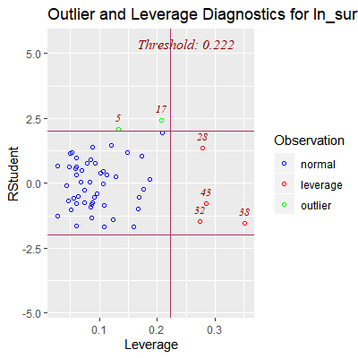
#obs 5 and 17 may be outlying wrt to Y
#obs 28, 32, 38, and 28 are outlying wrt to X


#check to see if these obs are influential

#to plot dffits
ols_plot_dffits(fit)




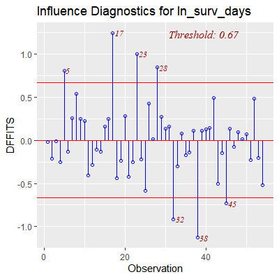
#obs 5, 17 28, 32, and 38 are outliers and influential 
#to their own fitted values

#plot Cook's distance
ols_plot_cooksd_chart(fit)




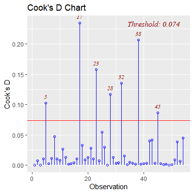
#obs 5, 17 28, 32, and 38 are outliers and influential 
#to all the fitted values

#plot dfbetas
ols_plot_dfbetas(fit)





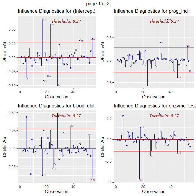
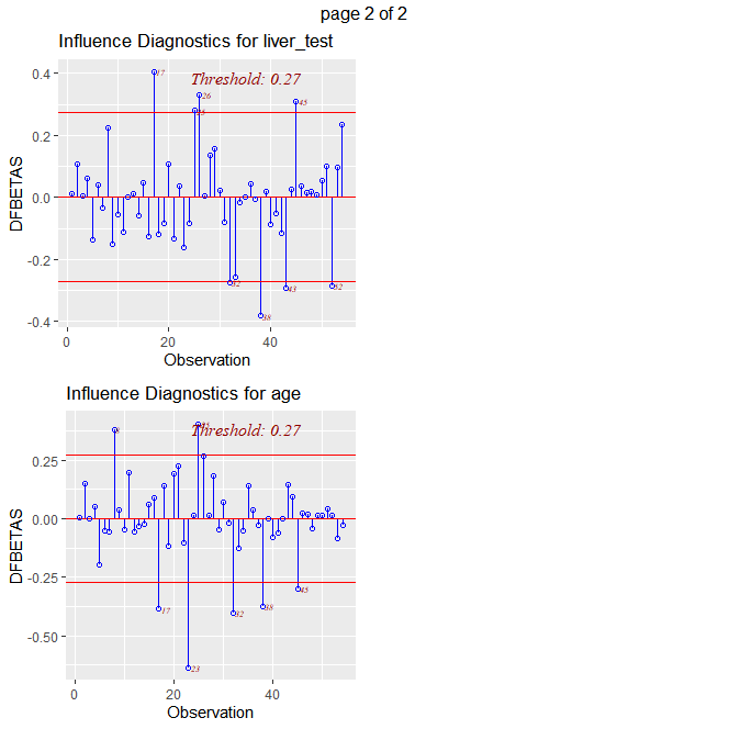
# obs 5 is influential on blood_clot and enzyme test
# obs 17 is influential on blood_clot, enzyme test, liver test, and age
# obs 28 is influential on blood_clot
# obs 32 is influential on prog_ind, enzyme test, liver_test, and age
# obs 38 is influential on prog_ind, blood clot, liver test, and age

# these five observations are outliers and influential to the fit. 
# They should all be examined to decide if a remedial measure is necessary.

« 5.2: Adding a Predictor Variable 5.4: Residual Diagnostics »