7.1 Model Selection Criteria

Thus far, we have discussed all steps except for step 3 (potential subsets of predictor variables) and step 8 (model validation).

We will discuss how to do these in this chapter. We start by discussing the criteria that could be used for comparing different models.

From any set of $p - 1$ predictors, $2^{p-1}$ alternative models can be constructed.

This calculation is based on the fact that each predictor can be either included or excluded from the model.

For example, the $$ 2^4 = 16 $$ different possible subset models that can be formed from the pool of four $X$ variables are $$ \begin{align*} & \text{None}\\ & X_{1}\\ & X_{2}\\ & X_{3}\\ & X_{4}\\ & X_{1},X_{2}\\ & X_{1},X_{3}\\ & X_{1},X_{4}\\ & X_{2},X_{3}\\ & X_{2},X_{4}\\ & X_{3},X_{4}\\ & X_{1},X_{2},X_{3}\\ & X_{1},X_{2},X_{4}\\ & X_{1},X_{3},X_{4}\\ & X_{2},X_{3},X_{4}\\ & X_{1},X_{2},X_{3},X_{4} \end{align*} $$ If there are 10 potential predictor variables, there there would be $$ 2^{10} = 1024 $$ possible subset models.

Model selection procedures, also known as subset selection or variables selection procedures, have been developed to identify a small group of regression models that are "good" according to a specified criterion.

This limited number might consist of three to six "good" subsets according to the criteria specified, so the investigator can then carefully study these regression models for choosing the final model.

While many criteria for comparing the regression models have been developed, we will focus on six: $$ \begin{align*} & R_{p}^{2}\\ & R_{a,p}^{2}\\ & C_{p}\\ & AIC_{p}\\ & SBC_{p}\\ & PRESS_{p} \end{align*} $$

Before discussing the criteria, we will need to develop some notation. We will denote the number of potential $X$ variables in the pool by $P-1$.

We assume that all regression models contain an intercept term $\beta_0$.

Hence, the regression function containing all potential $X$ variables contains $P$ parameters, and the function with no $X$ variables contains one parameter ($\beta_0$).

The number of $X$ variables in a subset will be denoted by $p-1$, as always, so that there are $p$ parameters in the regression function for this subset of $X$ variables. Thus, we have: $$ 1\le p \le P < n $$

Clearly, we would like models that fit the data well. Thus we would like a coefficient of multiple determiantion, $R^2$, to be high.

We will denote the number of parameters in the potential model as a subscript and write the coefficient of determination as $R^2_p$.

The $R^2_p$ criterion is equivalent to using the error sum of squares $SSE_p$ as the criterion.

The $R^2_p$ criterion is not intended to identify the subsets that maximize this criterion.

We know that $R^2_p$ can never decrease as additional X variables are included in the model.

Hence, $R^2_p$ will be a maximum when all $P - 1$ potential X variables are included in the regression model.

The intent in using the $R^2_p$ criterion is to find the point where adding more $X$ variables is not worthwhile because it leads to a very small increase in $R^2_p$.

Often, this point is reached when only a limited number of X variables is included in the regression model.

Since $R^2_{p}$ does not take account of the number of parameters in the regression model and since max($R^2_{p}$) can never decrease as $p$ increases, the adjusted coefficient of multiple determination $R^2_{a,p}$ has been suggested as an alternative criterion.

This coefficient takes the number of parameters in the regression model into account through the degrees of freedom.

Users of the $R^2_{a,p}$ criterion seek to find a few subsets for which $R^2_{a,p}$ is at the maximum or so close to the maximum that adding more variables is not worthwhile.

The $R^2_{a,p}$ criterion is equivalent to using the mean square error $SSE_p$ as the criterion. This come from the relationship in (4.44) \begin{align*} R_{a}^{2} & =1-\frac{\frac{SSE}{n-p}}{\frac{SSTO}{n-1}}\\ & =1-\left(\frac{n-1}{n-p}\right)\frac{SSE}{SSTO}\qquad(4.44)\\ & = 1-\frac{MSE}{\frac{SSTO}{n-1}} \end{align*}

We have seen that $R_{a,p}^2$ is a criterion that penalizes models having large numbers of predictors.

Two popular alternatives that also provide penalties for adding predictors are Akaike's information criterion ($AIC_p$) and Schwarz' Bayesian criterion ($SBC_p$).

A more popular name for $SBC_p$ is Bayesian information criterion ($BIC_p$).

We search for models that have small values of $AIC_p$, or $BIC_p$, where these criteria are given by: $$ \begin{align*} AIC_{p} & =n\ln SSE_{p}-n\ln n+2p\qquad\qquad (7.1)\\ BIC_{p} & =n\ln SSE_{p}-n\ln n+\left(\ln n\right)p\qquad (7.2) \end{align*} $$ Notice that for both of these measures, the first term is $$ n\ln SSE_{p} $$ which decreases as $p$ increases.

The second term is fixed (for a given sample size $n$), and the third term increases with the number of parameters, $p$.

Models with small $SSE_p$ will do well by these criteria as long as the penalties $$ \begin{align*} 2p & \text{ for }AIC_p \\ (\ln n)p & \text{ for }BIC_p \end{align*} $$ are not too large.

If $n \ge 8$ the penalty for $BIC_p$ is larger than that for $AIC_p$; hence the $BIC_p$ criterion tends to favor more parsimonious models.

A parsimonious model is a model that accomplishes a desired level of explanation or prediction with as few predictor variables as possible.

We consider the "best" models the ones with the lowest $AIC_p$ or $BIC_p$.

This criterion is concerned with the total mean squared error of the $n$ fitted values for each subset regression model.

The mean squared error concept involves the total error in each fitted value: $$ \hat{Y}_i-\mu_i $$ where $\mu_i$ is the true mean response when the levels of the predictor variables are those for the $i$th case.

This mean squared error involves two components which is related to the bias-variance tradeoff briefly mentioned in Section 5.5.4. Here, the mean square error is \begin{align*} E\left[\hat{Y}_{i}-\mu_{i}\right]^{2} & =\left(E\left[\hat{Y}_{i}\right]-\mu_{i}\right)^{2}+Var\left[\hat{Y}_{i}\right]\qquad(7.3) \end{align*} The quantity $E\left[\hat{Y}_{i}-\mu_{i}\right]^{2}$ is the mean squared error, $E\left[\hat{Y}_{i}\right]-\mu_{i}$ is the bias, and $Var\left[\hat{Y}_{i}\right]$ is the variance.

The total mean squared error for all $n$ fitted values is the sum of the $n$ individual mean squared errors: $$ \sum_{i=1}^n \left(E\left[(\hat{Y}_i-\mu_i)^2\right]\right)=\sum_{i=1}^nVar\left[\hat{Y}_i\right]+\sum_{i=1}^n\left(E\left[\hat{Y}_i\right]-\mu_i\right)^2\qquad(7.4) $$ If we divide (7.4) by $\sigma^2$, then we have the quantity \begin{align*} \Gamma_{p} & =\frac{1}{\sigma^{2}}\left[\sum_{i=1}^{n}\left(E\left[\hat{Y}_{i}\right]-\mu_{i}\right)^{2}+\sum_{i=1}^{n}Var\left[\hat{Y}_{i}\right]\right]\qquad(7.5) \end{align*} The model which includes all $P-1$ potential $X$ variables is assumed to have been carefully chosen so that $ MSE\left(X_1,\ldots,X_{P-1}\right) $ is an unbiased estimator of $\sigma^2$.

It can then be shown that an estimator of $\Gamma_p$ is $$ C_p = \frac{SSE_p}{MSE\left(X_1,\ldots,X_{P-1}\right)}-(n-2p)\qquad (7.6) $$ where $SSE_p$ is the error sum of squares for the fitted subset regression model with $p$ parameters. This criterion is called Mallows' $C_p$.

When there is no bias in the regression model with $p - 1$ $X$ variables so that $E[\hat{Y}_i]=\mu_i$, the expected value of $C_p$ is approximately $p$: $$ E[C_p]\approx p $$ Thus, when the $C_p$ values for all possible regression models are plotted against $p$, those models with little bias will tend to fall near the line $C_p = p$.

Models with substantial bias will tend to fall considerably above this line.

$C_p$ values below the line $C_p = p$ are interpreted as showing no bias, being below the line due to sampling error.

The $C_p$ value for the regression model containing all $P - 1$ $X$ variables is, by definition, $P$.

In using the $C_p$ criterion, we seek to identify subsets of $X$ variables for which

1. the $C_p$ value is small and
2. the $C_p$ value is near $p$.

Subsets with small $C_p$ values have a small total mean squared error, and when the $C_p$ value is also near $p$, the bias of the regression model is small.

It may sometimes occur that the regression model based on a subset of $X$ variables with a small $C_p$ value involves substantial bias. In that case, one may at times prefer a regression model based on a somewhat larger subset of $X$ variables for which the $C_p$ value is only slightly larger but which does not involve substantial bias.

The $PRESS_p$ (prediction sum of squares) criterion is a measure of how well the use of the fitted values for a subset model can predict the observed responses $Y_i$.

The PRESS measure differs from SSE in that each fitted value $\hat{Y}_i$ for the PRESS criterion is obtained by
1. deleting the $i$th case from the data set
2. estimating the regression function for the subset model from the remaining $n - 1$ cases, and
3. then using the fitted regression function to obtain the predicted value $\hat{Y}_{i(i)}$ for the $i$th case.

We use the notation $\hat{Y}_{i(i)}$ now for the fitted value to indicate, by the first subscript $i$, that it is a predicted value for the $i$th case and, by the second subscript $(i)$, that the $i$th case was omitted when the regression function was fitted.

The PRESS prediction error for the $i$th case then is: $$ Y_i - \hat{Y}_{i(i)} $$ and the $PRESS_p$ criterion is the sum of the squared prediction errors over all $n$ cases: $$ PRESS_p = \sum_{i=1}^n\left(Y_i - \hat{Y}_{i(i)} \right)^2\qquad (7.7) $$ Models with small $PRESS_p$ values are considered good candidate models. The reason is that when the prediction errors $Y_i - \hat{Y}_{i(i)}$ are small, so are the squared prediction errors and the sum of the squared prediction errors.

Thus, models with small $PRESS_p$ values fit well in the sense of having small prediction errors.

Another measure of prediction is the predicted $R^{2}$. Is is related to PRESS by \begin{align*} \text{pred }R_{p}^{2} & =1-\frac{PRESS_{p}}{SSTO}\qquad (7.8) \end{align*} Large values of ped $R_{p}^{2}$ indicates a model that is ``good'' at prediction.

Let's examine the surgical unit data from Example 5.3.2

library(tidyverse)
library(olsrr)

dat = read.table("http://www.jpstats.org/Regression/data/surgicalunit.txt", header=T)
dat$surv_days=NULL


#fit the full model
full = lm(ln_surv_days~., data=dat)

#get R^2, adj R^2, AIc, BIC, Cp, 
subsets = ols_step_all_possible(full)


#get the top six models by R^2
subsets %>% arrange(desc(rsquare)) %>% select( mindex, n, predictors, rsquare) %>% head

  mindex n                                                              predictors   rsquare
1    255 8 blood_clot prog_ind enzyme_test liver_test age gender alc_mod alc_heavy 0.8461286
2    247 7            blood_clot prog_ind enzyme_test age gender alc_mod alc_heavy 0.8460279
3    248 7         blood_clot prog_ind enzyme_test liver_test age gender alc_heavy 0.8436146
4    219 6                    blood_clot prog_ind enzyme_test age gender alc_heavy 0.8434363
5    249 7     blood_clot prog_ind enzyme_test liver_test gender alc_mod alc_heavy 0.8403866
6    250 7        blood_clot prog_ind enzyme_test liver_test age alc_mod alc_heavy 0.8395587


#get the top six models by adj R^2
subsets %>% arrange(desc(adjr)) %>% select( mindex, n, predictors, adjr) %>% head

  mindex n                                                              predictors      adjr
1    219 6                    blood_clot prog_ind enzyme_test age gender alc_heavy 0.8234494
2    247 7            blood_clot prog_ind enzyme_test age gender alc_mod alc_heavy 0.8225974
3    163 5                        blood_clot prog_ind enzyme_test gender alc_heavy 0.8205081
4    248 7         blood_clot prog_ind enzyme_test liver_test age gender alc_heavy 0.8198168
5    255 8 blood_clot prog_ind enzyme_test liver_test age gender alc_mod alc_heavy 0.8187737
6    164 5                           blood_clot prog_ind enzyme_test age alc_heavy 0.8187050


#get the top six models by AIC
subsets %>% arrange(aic) %>% select( mindex, n, predictors, aic) %>% head

  mindex n                                                   predictors       aic
1    219 6         blood_clot prog_ind enzyme_test age gender alc_heavy -8.588928
2    163 5             blood_clot prog_ind enzyme_test gender alc_heavy -8.559813
3     93 4                    blood_clot prog_ind enzyme_test alc_heavy -8.105992
4    164 5                blood_clot prog_ind enzyme_test age alc_heavy -8.020058
5    247 7 blood_clot prog_ind enzyme_test age gender alc_mod alc_heavy -7.490288
6    165 5         blood_clot prog_ind enzyme_test liver_test alc_heavy -7.149536


#get the top six models by BIC
subsets %>% arrange(sbc) %>% select( mindex, n, predictors, sbc) %>% head

  mindex n                                           predictors      sbc
1     93 4            blood_clot prog_ind enzyme_test alc_heavy 3.827912
2    163 5     blood_clot prog_ind enzyme_test gender alc_heavy 5.363075
3    164 5        blood_clot prog_ind enzyme_test age alc_heavy 5.902830
4    165 5 blood_clot prog_ind enzyme_test liver_test alc_heavy 6.773352
5    166 5    blood_clot prog_ind enzyme_test alc_mod alc_heavy 7.245232
6    219 6 blood_clot prog_ind enzyme_test age gender alc_heavy 7.322944


#get the top six models by cp
subsets %>% arrange(abs(cp-n+1)) %>% select( mindex, n, predictors, cp) %>% head

  mindex n                                                              predictors       cp
1    219 6                    blood_clot prog_ind enzyme_test age gender alc_heavy 5.787389
2    247 7            blood_clot prog_ind enzyme_test age gender alc_mod alc_heavy 7.029455
3    163 5                        blood_clot prog_ind enzyme_test gender alc_heavy 5.540639
4    248 7         blood_clot prog_ind enzyme_test liver_test age gender alc_heavy 7.735230
5    255 8 blood_clot prog_ind enzyme_test liver_test age gender alc_mod alc_heavy 9.000000
6    164 5                           blood_clot prog_ind enzyme_test age alc_heavy 6.018212


#get the top six models by pred R^2
subsets %>% arrange(desc(predrsq)) %>% select( mindex, n, predictors, predrsq) %>% head

  mindex n                                            predictors   predrsq
1     93 4             blood_clot prog_ind enzyme_test alc_heavy 0.7862406
2    164 5         blood_clot prog_ind enzyme_test age alc_heavy 0.7861500
3    219 6  blood_clot prog_ind enzyme_test age gender alc_heavy 0.7835427
4    222 6 blood_clot prog_ind enzyme_test age alc_mod alc_heavy 0.7830792
5    163 5      blood_clot prog_ind enzyme_test gender alc_heavy 0.7827317
6    166 5     blood_clot prog_ind enzyme_test alc_mod alc_heavy 0.7817215



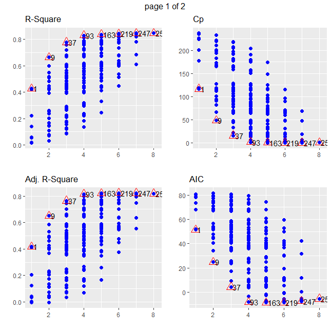
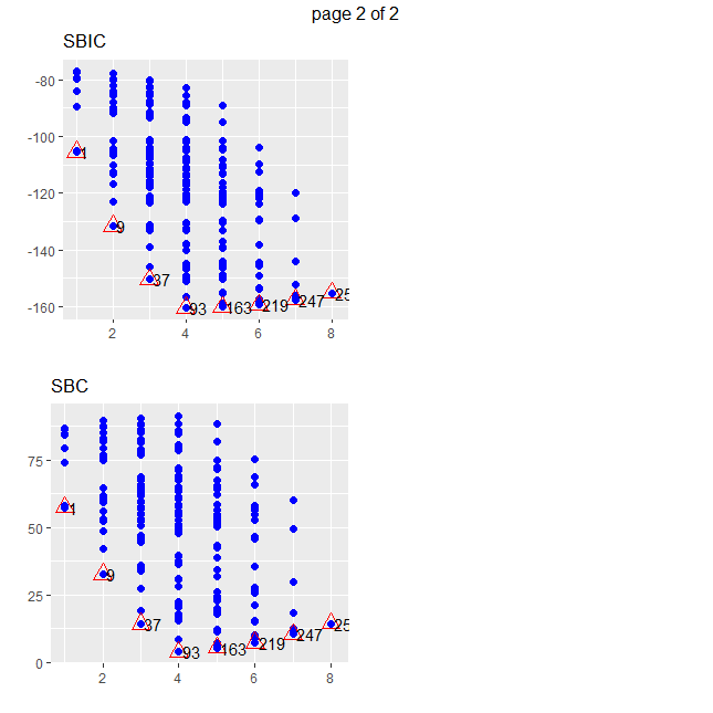
#visualize the model selection criteria
plot(subsets)