Fill in Blanks
Home
1.1 Bivariate Relationships
1.2 Probabilistic Models
1.3 Estimation of the Line
1.4 Properties of the Least Squares Estimators
1.5 Estimation of the Variance
2.1 The Normal Errors Model
2.2 Inferences for the Slope
2.3 Inferences for the Intercept
2.4 Correlation and Coefficient of Determination
2.5 Estimating the Mean Response
2.6 Predicting the Response
3.1 Residual Diagnostics
3.2 The Linearity Assumption
3.3 Homogeneity of Variance
3.4 Checking for Outliers
3.5 Correlated Error Terms
3.6 Normality of the Residuals
4.1 More Than One Predictor Variable
4.2 Estimating the Multiple Regression Model
4.3 A Primer on Matrices
4.4 The Regression Model in Matrix Terms
4.5 Least Squares and Inferences Using Matrices
4.6 ANOVA and Adjusted Coefficient of Determination
4.7 Estimation and Prediction of the Response
5.1 Multicollinearity and Its Effects
5.2 Adding a Predictor Variable
5.3 Outliers and Influential Cases
5.4 Residual Diagnostics
5.5 Remedial Measures
6.2 Interaction Between Predictors
"Back off man, I'm a Scientist."
- Peter Venkman (Ghostbusters)
There are instances in which the effects of the different predictor
variables on $Y$ are not additive. Instead, the effect of one predictor
variable depends on the levels of the other predictor variables.
For example, suppose we have two predictor variables $X_{1}$ and $X_{2}$. A model that takes into account theinteraction between
the levels of the two variables is
\begin{align*}
Y_{i} & =\beta_{0}+\beta_{1}X_{i1}+\beta_{2}X_{i2}+\beta_{3}X_{i1}X_{i2}+\varepsilon_{i}\qquad(6.1)
\end{align*}
We call the term $\beta_{3}X_{i1}X_{i2}$ an interaction term .
We can let $X_{i3}=X_{i1}X_{i2}$ and then rewrite the model as \begin{align*} Y_{i} & =\beta_{0}+\beta_{1}X_{i1}+\beta_{2}X_{i2}+\beta_{3}X_{i3}+\varepsilon_{i} \end{align*} We could have three predictor variables whose levels affect each other. This would mean there are \begin{align*} \binom{3}{2} & =\frac{3!}{2!\left(3-2\right)!}=3 \end{align*} possible interaction terms. The model with interaction terms for all possible pairs would be \begin{align*} Y_{i} & =\beta_{0}+\beta_{1}X_{i1}+\beta_{2}X_{i2}+\beta_{3}X_{i3}+\beta_{4}X_{i1}X_{i2}+\beta_{5}X_{i1}X_{i3}+\beta_{6}X_{i2}X_{i3}+\varepsilon_{i} \end{align*}
For example, suppose we have two predictor variables $X_{1}$ and $X_{2}$. A model that takes into account the
We can let $X_{i3}=X_{i1}X_{i2}$ and then rewrite the model as \begin{align*} Y_{i} & =\beta_{0}+\beta_{1}X_{i1}+\beta_{2}X_{i2}+\beta_{3}X_{i3}+\varepsilon_{i} \end{align*} We could have three predictor variables whose levels affect each other. This would mean there are \begin{align*} \binom{3}{2} & =\frac{3!}{2!\left(3-2\right)!}=3 \end{align*} possible interaction terms. The model with interaction terms for all possible pairs would be \begin{align*} Y_{i} & =\beta_{0}+\beta_{1}X_{i1}+\beta_{2}X_{i2}+\beta_{3}X_{i3}+\beta_{4}X_{i1}X_{i2}+\beta_{5}X_{i1}X_{i3}+\beta_{6}X_{i2}X_{i3}+\varepsilon_{i} \end{align*}
When an interaction term is included in the model, the interpretation
of the coefficients are not the same as if there were no interaction
term. If there are no interaction terms in (6.1), then an increase
of $X_{1}$ by one unit, while holding $X_{2}$ constant, gives the
mean response as
\begin{align*}
E\left[Y\right] & =\beta_{0}+\beta_{1}\left(X_{1}+1\right)+\beta_{2}X_{2}
\end{align*}
The change in the mean response from when $X_{1}$ increases to $X_{1}+1$
gives
\begin{align*}
& \beta_{0}+\beta_{1}X_{1}+\beta_{2}X_{2}-\left[\beta_{0}+\beta_{1}\left(X_{1}+1\right)+\beta_{2}X_{2}\right]\\
& =\beta_{1}
\end{align*}
If an interaction term is in equation (6.1), then the mean response
when $X_{1}$ is increased by one unit, while holding $X_{2}$ constant,
is
\begin{align*}
E\left[Y\right] & =\beta_{0}+\beta_{1}\left(X_{1}+1\right)+\beta_{2}X_{2}+\beta_{3}\left(X_{1}+1\right)X_{2}\\
& =\beta_{0}+\beta_{1}\left(X_{1}+1\right)+\beta_{2}X_{2}+\beta_{3}X_{1}X_{2}+\beta_{3}X_{2}
\end{align*}
The change in the mean response from when $X_{1}$ increases to $X_{1}+1$
is then
\begin{align*}
& \beta_{0}+\beta_{1}X_{1}+\beta_{2}X_{2}+\beta_{3}X_{1}X_{2}-\left[\beta_{0}+\beta_{1}\left(X_{1}+1\right)+\beta_{2}X_{2}+\beta_{3}X_{1}X_{2}+\beta_{3}X_{2}\right]\\
& =\beta_{1}+\beta_{3}X_{2}
\end{align*}
So the effect of $X_{1}$ for some fixed level of $X_{2}$ depends
on the level of $X_{2}$.
The same could be shown for the effect of $X_{2}$ on $Y$ for a fixed level of $X_{1}$.
The same could be shown for the effect of $X_{2}$ on $Y$ for a fixed level of $X_{1}$.
Interaction terms can also be used when the predictor variables are
qualitative. For instance, suppose $X_{2}$ is an indicator variable
for some dichotomous predictor in model (6.1).
When $X_{2}=$1, we then have \begin{align*} E\left[Y\right] & =\beta_{0}+\beta_{1}X_{1}+\beta_{2}\left(1\right)+\beta_{3}X_{1}\left(1\right)\\ & =\left(\beta_{0}+\beta_{2}\right)+\left(\beta_{1}+\beta_{3}\right)X_{1} \end{align*} When $X_{2}=0$, we have \begin{align*} E\left[Y\right] & =\beta_{0}+\beta_{1}X_{1}+\beta_{2}\left(0\right)+\beta_{3}X_{1}\left(0\right)\\ & =\beta_{0}+\beta_{1}X_{1} \end{align*} Thus, when $X_{2}=1$ we have a line that has a different intercept $\left(\beta_{0}+\beta_{2}\right)$ and different slope $\left(\beta_{1}+\beta_{3}\right)$ than when $X_{2}=0$.
When there is no interaction term included in the model, then we have a different intercept but the same slope as shown in Section 6.1.1.
When including interaction terms in the multiple regression model,
we should keep a couple considerations in mind.
First, when we fit the model we will use the least squares as we have done before by considering the interaction terms as just another variable. For instance, in model (6.1) above, we would consider $X_{i3}=X_{i1}X_{i2}$ and then include $X_{3}$ as a column in the design matrix ${\bf X}$.
Because of this, including an interaction term may introduce highmulticollinearity to the model.
Another consideration when including interaction terms is the potential for a large number of parameters that need to be estimated. For example, if we have six predictor variables and we want to include an interaction term for each pair of these six variables, we would then have \begin{align*} \binom{6}{2} & =\frac{6!}{2!\left(6-2\right)!}=15 \end{align*} coefficients for all of these pairs. That would mean the model would have a total of 22 coefficients to estimate (1 intercept, 6 coefficients for the predictor variables, and 15 coefficients for the interaction terms).
Because of the number of possible interaction terms, it is best to investigate the nature of the variables and interactions before attempting to model the variables. This could be done by using expert opinion from those who are familiar with the application.
One can also plot the residuals of the model with no interaction terms against the different interactions to determine if any appear influential on $Y$.
First, when we fit the model we will use the least squares as we have done before by considering the interaction terms as just another variable. For instance, in model (6.1) above, we would consider $X_{i3}=X_{i1}X_{i2}$ and then include $X_{3}$ as a column in the design matrix ${\bf X}$.
Because of this, including an interaction term may introduce high
Another consideration when including interaction terms is the potential for a large number of parameters that need to be estimated. For example, if we have six predictor variables and we want to include an interaction term for each pair of these six variables, we would then have \begin{align*} \binom{6}{2} & =\frac{6!}{2!\left(6-2\right)!}=15 \end{align*} coefficients for all of these pairs. That would mean the model would have a total of 22 coefficients to estimate (1 intercept, 6 coefficients for the predictor variables, and 15 coefficients for the interaction terms).
Because of the number of possible interaction terms, it is best to investigate the nature of the variables and interactions before attempting to model the variables. This could be done by using expert opinion from those who are familiar with the application.
One can also plot the residuals of the model with no interaction terms against the different interactions to determine if any appear influential on $Y$.
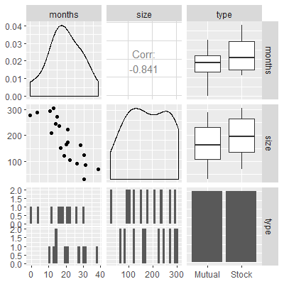
Data on the speed with which a particular insurance innovation is adopted (in months) along with the size of the insurance firm and type of firm can be found in insurance.txt which is from Kutner
An economists wants to model the number of elapsed months based on the size and type of the insurance firm.
Kutner, M. H., Nachtsheim, C. J., Neter, J., & Li, W. (2005). Applied linear statistical models (Vol. 5). Boston: McGraw-Hill Irwin.
.
An economists wants to model the number of elapsed months based on the size and type of the insurance firm.
library(tidyverse)
library(car)
library(olsrr)
library(MASS)
library(glmnet)
library(GGally)
dat = read.table("http://www.jpstats.org/Regression/data/insurance.txt", header=T)
#let's first visualize the data
ggpairs(dat)
#fit with no interaction term
fit = lm(months~size+type, data=dat)
fit %>% summary
Call:
lm(formula = months ~ size + type, data = dat)
Residuals:
Min 1Q Median 3Q Max
-5.6915 -1.7036 -0.4385 1.9210 6.3406
Coefficients:
Estimate Std. Error t value Pr(>|t|)
(Intercept) 33.874069 1.813858 18.675 9.15e-13 ***
size -0.101742 0.008891 -11.443 2.07e-09 ***
typeStock 8.055469 1.459106 5.521 3.74e-05 ***
---
Signif. codes:
0 ‘***’ 0.001 ‘**’ 0.01 ‘*’ 0.05 ‘.’ 0.1 ‘ ’ 1
Residual standard error: 3.221 on 17 degrees of freedom
Multiple R-squared: 0.8951, Adjusted R-squared: 0.8827
F-statistic: 72.5 on 2 and 17 DF, p-value: 4.765e-09
#check to see if there is any multicollinearity
vif(fit)
size type
1.025951 1.025951
#we now want to plot the residuals vs
#the interaction
#first, we need to make type into an indicator
x3 = model.matrix(~dat$type)[,2]
#we now make a new variable as the product of
#size and type
dat$interaction = dat$size*x3
dat$e = fit %>% resid
ggplot(dat=dat, aes(x=interaction, y= e))+
geom_point()
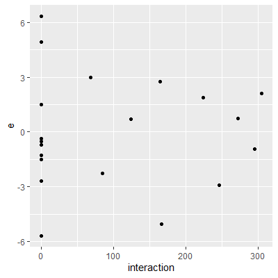
#there is no clear pattern in the plot so it appears
#there is no significant interaction between size
#and type
#if we wanted to fit the model with the interaction,
#we would do so in lm below:
fit2 = lm(months~size+type + size*type, data=dat)
fit2 %>% summary
Call:
lm(formula = months ~ size + type + size * type, data = dat)
Residuals:
Min 1Q Median 3Q Max
-5.7144 -1.7064 -0.4557 1.9311 6.3259
Coefficients:
Estimate Std. Error t value Pr(>|t|)
(Intercept) 33.8383695 2.4406498 13.864 2.47e-10 ***
size -0.1015306 0.0130525 -7.779 7.97e-07 ***
typeStock 8.1312501 3.6540517 2.225 0.0408 *
size:typeStock -0.0004171 0.0183312 -0.023 0.9821
---
Signif. codes:
0 ‘***’ 0.001 ‘**’ 0.01 ‘*’ 0.05 ‘.’ 0.1 ‘ ’ 1
Residual standard error: 3.32 on 16 degrees of freedom
Multiple R-squared: 0.8951, Adjusted R-squared: 0.8754
F-statistic: 45.49 on 3 and 16 DF, p-value: 4.675e-08
#we could now look at the t-test and see if the
#coefficient is significantly different from zero
#here, the t-test is insignificant. We must be careful
#since the t-test cold be affected by multicollinearity
#If there is multicollinearity, then the affect could
#be significant but the t-test shows insignificant
#if the t-test does show a significant result, then
#it is clear evidence of a significant effect since
#multicollinearity causes a larger type II error, not
#larger type I error
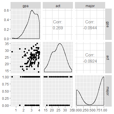
The gpa2 dataset consists of grade point average at the end of freshmen year, the ACT score, and an indicator variable for whether the student declares a major at the time of application or not.
The dataset can be found in Kutner
The dataset can be found in Kutner
Kutner, M. H., Nachtsheim, C. J., Neter, J., & Li, W. (2005). Applied linear statistical models (Vol. 5). Boston: McGraw-Hill Irwin.
. We wish to model gpa based on the other two variables.
library(tidyverse)
library(car)
library(olsrr)
library(MASS)
library(glmnet)
library(GGally)
dat = read.table("http://www.jpstats.org/Regression/data/gpa2.txt", header=T)
ggpairs(dat)
#fit with no interaction
fit = lm(gpa~act+major, data=dat)
fit %>% summary
Call:
lm(formula = gpa ~ act + major, data = dat)
Residuals:
Min 1Q Median 3Q Max
-2.70304 -0.35574 0.02541 0.45747 1.25037
Coefficients:
Estimate Std. Error t value Pr(>|t|)
(Intercept) 2.19842 0.33886 6.488 2.18e-09 ***
act 0.03789 0.01285 2.949 0.00385 **
major -0.09430 0.11997 -0.786 0.43341
---
Signif. codes:
0 ‘***’ 0.001 ‘**’ 0.01 ‘*’ 0.05 ‘.’ 0.1 ‘ ’ 1
Residual standard error: 0.6241 on 117 degrees of freedom
Multiple R-squared: 0.07749, Adjusted R-squared: 0.06172
F-statistic: 4.914 on 2 and 117 DF, p-value: 0.008928
vif(fit)
act major
1.00861 1.00861
#examine interaction
dat$interaction = dat$act*dat$major
dat$e = fit %>% resid
ggplot(dat=dat, aes(x=interaction, y= e))+
geom_point()
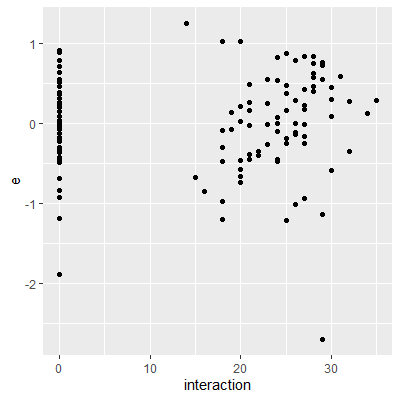
#it appears the may be some significant
#relationship between Y and the interaction
fit2 = lm(gpa~act+major+act*major, data=dat)
fit2 %>% summary
Call:
lm(formula = gpa ~ act + major + act * major, data = dat)
Residuals:
Min 1Q Median 3Q Max
-2.80187 -0.31392 0.04451 0.44337 1.47544
Coefficients:
Estimate Std. Error t value Pr(>|t|)
(Intercept) 3.226318 0.549428 5.872 4.18e-08 ***
act -0.002757 0.021405 -0.129 0.8977
major -1.649577 0.672197 -2.454 0.0156 *
act:major 0.062245 0.026487 2.350 0.0205 *
---
Signif. codes:
0 ‘***’ 0.001 ‘**’ 0.01 ‘*’ 0.05 ‘.’ 0.1 ‘ ’ 1
Residual standard error: 0.6124 on 116 degrees of freedom
Multiple R-squared: 0.1194, Adjusted R-squared: 0.09664
F-statistic: 5.244 on 3 and 116 DF, p-value: 0.001982
#here we see a significant interaction term