7.2 Best Subsets Procedure

"Everthing should be as simple as possible, but no simpler."
- Albert Einstein

7.2.1 Best Subsets Algorithm

As noted in the previous section, the number of possible models, $$ 2^{p-1} $$ grows rapidly with the number of predictors.

Evaluating all of the possible alternatives can be a daunting endeavor. To simplify the task, a variety of automatic computer-search procedures have been developed.

In this section, we will review one approach called best subsets regression.

Time-saving algorithms have been developed in which the best subsets according to a specified criterion are identified without requiring the fitting of all of the possible subset regression models.

In fact, these algorithms require the calculation of only a small fraction of all possible regression models.

For instance, if the $C_p$ criterion is to be employed and the five best subsets according to this criterion are to be identified, these algorithms search for the five subsets of X variables with the smallest $C_p$ values using much less computational effort than when all possible subsets are evaluated.

These algorithms are called "best" subsets algorithms.

Not only do these algorithms provide the best subsets according to the specified criterion, but they often also identify several "good" subsets for each possible number of X variables in the model to give the investigator additional helpful information in making the final selection of the subset of predictor variables to be employed in the regression model.

When the pool of potential X variables is very large, say greater than 30 or 40, even the "best" subset algorithms may require excessive computer time.

Under these conditions, one of the stepwise regression procedures, described in the next section, may need to be employed to assist in the selection of predictor variables.

Example 7.2.1

Best subsets regression with the surgical unit data. We will use the leaps library.

library(tidyverse)
library(car)
library(olsrr)
library(leaps)

dat = read.table("http://www.jpstats.org/Regression/data/surgicalunit.txt", header=T)
dat$surv_days=NULL

#fit the full model
full = lm(ln_surv_days~., data=dat)

#get the three best models for each p by aic
subsets = regsubsets(ln_surv_days~., data=dat, nbest = 3)
(summ = subsets %>% summary)

Subset selection object
Call: regsubsets.formula(ln_surv_days ~ ., data = dat, nbest = 3)
8 Variables  (and intercept)
            Forced in Forced out
blood_clot      FALSE      FALSE
prog_ind        FALSE      FALSE
enzyme_test     FALSE      FALSE
liver_test      FALSE      FALSE
age             FALSE      FALSE
gender          FALSE      FALSE
alc_mod         FALSE      FALSE
alc_heavy       FALSE      FALSE
3 subsets of each size up to 8
Selection Algorithm: exhaustive
         blood_clot prog_ind enzyme_test liver_test age gender alc_mod alc_heavy
1  ( 1 ) " "        " "      "*"         " "        " " " "    " "     " "      
1  ( 2 ) " "        " "      " "         "*"        " " " "    " "     " "      
1  ( 3 ) " "        "*"      " "         " "        " " " "    " "     " "      
2  ( 1 ) " "        "*"      "*"         " "        " " " "    " "     " "      
2  ( 2 ) " "        " "      "*"         "*"        " " " "    " "     " "      
2  ( 3 ) "*"        " "      "*"         " "        " " " "    " "     " "      
3  ( 1 ) " "        "*"      "*"         " "        " " " "    " "     "*"      
3  ( 2 ) "*"        "*"      "*"         " "        " " " "    " "     " "      
3  ( 3 ) " "        "*"      "*"         "*"        " " " "    " "     " "      
4  ( 1 ) "*"        "*"      "*"         " "        " " " "    " "     "*"      
4  ( 2 ) " "        "*"      "*"         "*"        " " " "    " "     "*"      
4  ( 3 ) " "        "*"      "*"         " "        " " "*"    " "     "*"      
5  ( 1 ) "*"        "*"      "*"         " "        " " "*"    " "     "*"      
5  ( 2 ) "*"        "*"      "*"         " "        "*" " "    " "     "*"      
5  ( 3 ) "*"        "*"      "*"         "*"        " " " "    " "     "*"      
6  ( 1 ) "*"        "*"      "*"         " "        "*" "*"    " "     "*"      
6  ( 2 ) "*"        "*"      "*"         " "        " " "*"    "*"     "*"      
6  ( 3 ) "*"        "*"      "*"         "*"        " " "*"    " "     "*"      
7  ( 1 ) "*"        "*"      "*"         " "        "*" "*"    "*"     "*"      
7  ( 2 ) "*"        "*"      "*"         "*"        "*" "*"    " "     "*"      
7  ( 3 ) "*"        "*"      "*"         "*"        " " "*"    "*"     "*"      
8  ( 1 ) "*"        "*"      "*"         "*"        "*" "*"    "*"     "*" 


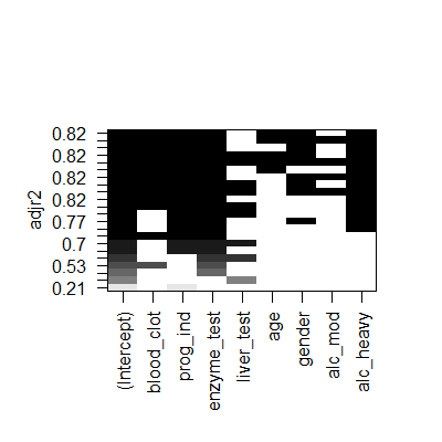
#visualize the model subsets
plot(subsets,scale = "adjr2")


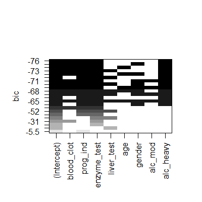
plot(subsets,scale = "bic")#actually aic


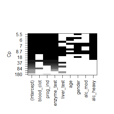
plot(subsets,scale = "Cp")


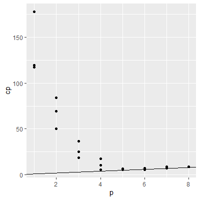
#a better plot for Mallow's Cp
cp.df = data.frame(p = summ$which %>% dimnames %>% .[[1]] %>% as.numeric,
                   cp = summ$cp)
ggplot(cp.df, aes(x=p, y=cp))+
  geom_point() +
  geom_abline(intercept = 0, slope=1)


#to compare computation time for examining all possible 
#subsets in ols_step_best_subset
#versus the algorithm only looking at the 3 best
#for each p in regsubsets
system.time(ols_step_best_subset(full))

   user  system elapsed 
   7.98    0.00    8.08

system.time(regsubsets(ln_surv_days~., data=dat, nbest = 3))

   user  system elapsed 
      0       0       0

7.2.2 Choosing a Subset of Models

The best subsets regressions procedure leads to the identification of a small number of subsets that are "good" according to a specified criterion.

Sometimes, one may wish to consider more than one criterion in evaluating possible subsets of predictor variables.

Once the investigator has identified a few "good" subsets for intensive examination, a final choice of the model variables must be made.

This choice is aided by examining outliers, checking model assumptions, and by the investigator's knowledge of the subject under study, and is finally confirmed through model validation studies.

« 7.1: Model Selection Criteria 7.3 Stepwise Regression Procedures »